Lombardi Drawings

Mark Lombardi (1951–2000) was an American artist whose network diagrams, like the one below, reveal close connections between actors in the domains of international politics and finance. In this post we examine recent work to emulate the aesthetic qualities of Lombardi’s drawings in the realm of graph drawing. More information about Mark Lombardi can be found in the papers (missing reference) and (missing reference) and in this story from a 2003 episode of Morning Edition on NPR.

Lombardi’s diagrams have very strong aesthetic qualities. These qualities have been attributed, in part, to his use of circular arcs for edges as well as his efforts to achieve equal spacing of edges around node perimeters; so-called perfect angular resolution.

In (missing reference) the notion of a Lombardi drawing of a graph is introduced. Such a drawing has perfect angular resolution as well as circular arc edges. The authors describe several methods for finding Lombardi drawings of graphs and they introduce a Python program called the Lombardi Spirograph which can produce Lombardi drawings of graphs.

In this post we will demonstrate how to use the Lombardi Spirograph to draw certain named graphs, how to use options to customise drawings and we will give two examples of the special input language for drawing graphs other than named ones.

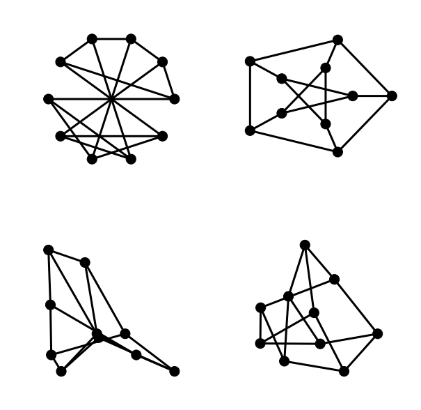
Below is a selection of a few of the smaller named graphs that can be drawn by the Lombardi Spirograph. To view other drawings, use the left and right arrow keys.

Drawing Named Graphs

The basic usage pattern for the Lombardi Spirograph is:

$ python LombardiSpirograph.py [options] graph_name > output.svg

where graph_name is to be replaced by either one of the names of the known named graphs or by a description of a graph using the specialist input language.

For example, to draw the Grötzsch graph with the default options:

$ python LombardiSpirograph.py grotzsch > grotzsch.svg

Which results in the following drawing:

Below is a slideshow of the remaining named graphs that can be drawn by the Lombardi Spirograph. Graph names can be deduced from the captions by removing all whitespace and changing all uppercase characters to lowercase.

Options

The Lombardi Spirograph allows customisation of several aspects of the produced drawing. We can scale the drawing and choose different styling options for the vertices: the colour, size and whether vertices have visible outlines or not. For example, to draw the Grötzsch graph again, slightly larger with smaller blue nodes not having visible outlines:

$ python LombardiSpirograph.py --scale=1.2 --color=blue --radius=0.8 --outline grotzsch > grotzsch_alt.svg

Drawing Other Graphs

The input language for drawing other graphs is described by the authors in the Lombardi Spirograph online documentation. The description can be read by running the program with the --format flag.

$ python LombardiSpirograph.py --format

The graph should be described as a sequence of alphanumeric words, separated either by spaces or by blank lines. The first word gives the order of symmetry of the drawing (the number of vertices in each concentric layer) and each subsequent word describes the vertices in a single layer of the graph.

Each word after the first takes the form of a (possibly empty) sequence of letters followed by a (possibly empty) number. The letters describe edges connecting two vertices in the same layer: “a” for a connection between consecutive vertices in the same layer, “b” for a connection between vertices two steps away from each other, etc. The letters should be listed in the order the connections should appear at the vertex, starting from the edge closest to the center of the drawing and progressing outwards. Only connections that span less than half the circle are possible, except that the first layer may have connections spanning exactly half the circle.

The numeric part of a word describes the connection from one layer to the next layer. If this number is zero, then vertices in the inner layer are connected to vertices in the next layer radially by straight line segments. Otherwise, pairs of vertices from the inner layer, the given number of steps apart, are connected to single vertices in the outer layer. A nonzero number written with a leading zero (e.g. “01” in place of “1”) indicates that, as well as connections with the given number of steps, there should also be a radial connection from the inner layer to the next layer that has vertices aligned with it; this may not necessarily be the layer immediately outward.

In the innermost layer, the special word “x” may be used to indicate that the layer consists of a single vertex at the center of the drawing. “x0” indicates that this central vertex is connected both to every vertex in the adjacent layer and also to every vertex in the next layer that is staggered with respect to the inner two layers.

Below are two examples. The icosahedron, which is one of the named graphs, and the Petersen graph, which is also named but in a different way than in the example below.

Example 1 – Icosahedron

A possible code for a Lombardi drawing of the icosahedron is 3-a01-01-1-a. The drawing that results is:

Here is how to interpret the graph description and see how the above drawing is produced from it.

• 3 - Gives the order of symmetry (vertices in each layer);
• a01 - describes connections with vertices in first (innermost) layer;
  • a - consecutive vertices in this layer are joined by an edge;
  • 01 - pairs of vertices one step apart in this layer are joined to vertices in the next layer and there are radial lines to the next aligned layer (in this case the third);
• 01 - pairs of vertices in second layer which are one step apart in this layer are joined to vertices in the next layer and there are radial lines to the next aligned layer (the fourth);
• 1 - pairs of vertices in second layer which are one step apart in this layer are joined to vertices in the next layer;
• a - consecutive vertices in fourth (outermost) layer are joined by an edge.

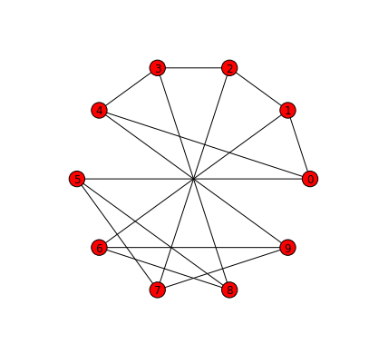
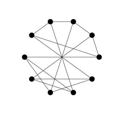
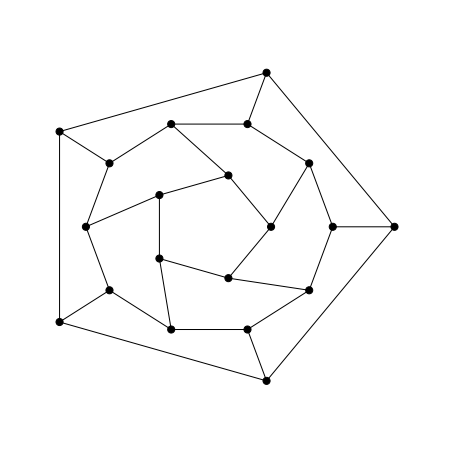
Example 2 – The Petersen Graph

According to the above description we can deduce that 5-b0-a is a representation of a drawing of the Petersen graph. The drawing produced by the Lombardi Spirograph is shown below.

References

Basic Graph Drawing

In this post we introduce the drawing functionality of NetworkX.

This post is also available as a notebook for IPython which can be viewed online here.

1. Basic Drawing

All drawing in NetworkX can handled by the draw function. Layouts are generated using functions like circular_layout and spring_layout which return coordinate mappings that can be used by the draw function to render the graph.

In addition, every layout algorithm also has its own convenience function. For example, the circular layout method can be used by calling the draw_circular function and the spring layout method can be used through the draw_spring function.

In this section we will demonstrate how to use both the draw function and the different layout functions.

As with all work involving NetworkX, we have to start by importing the package. We choose to follow the popular convention to import network as nx.

import networkx as nx

NetworkX makes many named graphs available. For example, the Petersen Graph can be generated by calling the petersen_graph function.

G = nx.petersen_graph()

One way to draw the Petersen Graph with a circular layout is to pass the draw function a parameter giving the coordinates of the vertices in a circular layout. These coordinates are the output of the circular_layout function which takes the graph as a parameter.

nx.draw(G, nx.circular_layout(G))

Instead of using the draw function in conjunction with the circular_layout function we can use the draw_circular convenience function.

The draw function and all of the layout convenience functions can be configured to produce graph drawings with different visual properties. Keyword parameters can be specified to customise things like node colours, edge widths and whether the graph is displayed with labels or not.

A list of all node properties that can be configured is here. A list of all edge properties that can be configured is here.

nx.draw_circular(G, with_labels=False, node_color='black')

As these configuration options are going to be used on several graphs it makes sense to put all of the option configurations into a dictionary and then pass the dictionary as a parameter to the relevant layout function.

options = {
 'with_labels': False,
 'node_color': 'black',
 'node_size': 200,
 'width': 3,
}

nx.draw_circular(G, **options)

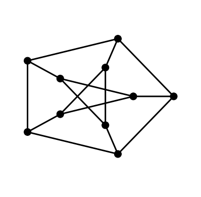
This drawing is not so easily recognised as a drawing of the Petersen Graph. A more familiar drawings shows one of the five cycles in the shape of a regular pentagon with another five cycle as a star in the interior joined to the outer cycle by five spokes. We can achieve this layout in NetworkX with the shell layout algorithm.

The draw_shell function takes an optional nlist keyword argument. The elements of the list are lists of vertices. The vertices are then arranged in concentric shells according to the elements of these lists. To find which vertices lie in the outer shell and which are in the inner shell, along with their respective orderings requires some experimentation.

nx.draw_shell(G, nlist=[range(5,10), range(5)], **options)

2. Simple Layouts - graphs with few vertices

NetworkX has the following layout algorithms.

• Circular
• Shell
• Spring
• Spectral
• Random
• Graphviz (through pygraphviz)

We have seen already examples of the circular and shell layouts. The next figure reproduces those two drawings from above along with examples of the spring and spectral layouts.

plt.subplot(221)
nx.draw_circular(G, **options)

plt.subplot(222)
nx.draw_shell(G, nlist=[range(5,10), range(5)], **options)

plt.subplot(223)
nx.draw_spectral(G, **options)

plt.subplot(224)
nx.draw_spring(G, **options)

The plt.subplot command will be familiar to anyone with Matlab experience. It takes an integer argument whose first two digits are interpreted as a number of rows and columns in a rectangular grid layout and whose third argument is interpreted as the position of the current figure in the grid. Grid numbering starts in the top-left corner and proceeds right and downwards to the bottom- right corner.

3. Graphs with a few more nodes

The options we have chosen so far have been suitable for graphs with a few nodes. When we are drawing larger graphs it makes sense to choose smaller node sizes and thinner edges so that the various elements of the graph can be easily distinguished.

options_1 = {
 'with_labels': False,
 'node_color': 'black',
 'node_size': 50,
 'width': 1,
}

As with the earlier drawing of the Petersen graph the nodes for the different layers of the drawing of the dodecahedral graph below were here figured out by manual experimentation.

G = nx.dodecahedral_graph()
nx.draw_shell(G, nlist = [[2,3,4,5,6],[8,1,0,19,18,17,16,15,14,7],[9,10,11,12,13]], **options_1)

4. Graphs with many more nodes

If a graph has many nodes then there is a risk, in particular with circular or shell layouts, that node boundaries can overlap. Choosing small node sizes is a natural remedy. But when choosing very small nodes edges must also be made very thin so that we can resolve node edge intersections. Thin edges look grey and then it is natural to choose grey nodes to match.

options_2 = {
 'with_labels': False,
 'node_color': 'grey',
 'node_size': 10,
 'linewidths': 0,
 'width': 0.1,
}

G = nx.barabasi_albert_graph(100, 3)
nx.draw_circular(G, **options_2)

5. Graphs with many edges

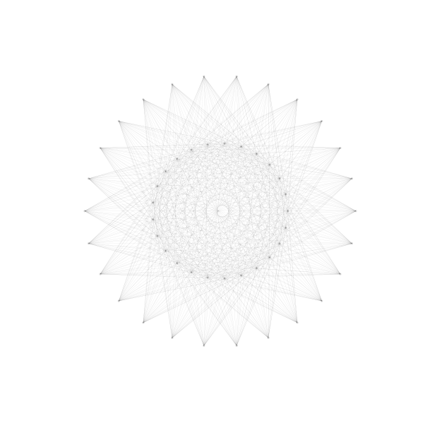
Drawing graphs with many edges requires further tinkering with layout options. A new problem in this situation is that edges cannot be easily distinguished or have end vertices that are difficult to recognise. Increasing transparency by lowering the alpha value may have some benefit here.

options_3 = {
 'with_labels': False,
 'node_color': 'grey',
 'node_size': 10,
 'linewidths': 0,
 'width': 0.1,
 'alpha': 0.3
}

G = nx.complete_bipartite_graph(25,26)
nx.draw_shell(G, nlist=[range(0,25), range(25,51)], **options_3)

Admittedly, this drawing conveys little information about the graph. It is hard even to see which nodes in the inner shell are connected to nodes in the outer shell or if there are any connections between nodes in the inner shell. About the only information we can interpret is that nodes in the outer shell appear not to be joined to other vertices in the outer shell. Still, it serves as a basic example of the kind of issues that we face when trying to draw graphs with many edges.

4. Importing layouts from Gephi

Naturally, some of the problems encountered above are due to poorly chosen layouts. Better layouts can reduce problems of identifying nodes and edges. Even better layouts can help to highlight structural properties and symmetries of graphs.

G = nx.random_lobster(100, 0.9, 0.9)
nx.draw_spring(G, iterations=10000, **options_2)

In a previous post we talked about how to use Gephi to find nice layouts of large lobster graphs. As an alternative to using NetworkX’s layout algorithms we can export our graph, use Gephi to find a suitable layout and then import the graph data back (now augmented with coordinate information) and use the raw drawing ability of NetworkX to render the graph with this layout.

G = nx.read_graphml('/home/matthew/tmp/lobster.graphml')
pos = dict([(v,(G.node[v]['x'], G.node[v]['y'])) for v in G.nodes()])

NetworkX loads the graph as a directed graph and will draw directed edges with arrows unless we set the arrows keyword argument to False.

nx.draw(G, pos, arrows=False, **options_2)

This drawing nearly has it all. The chosen layout almost conveys the planarity and lobsterity of the graph clearly. With a little manual adjustment we could eliminate all edge-crossings but because we value reproducibility above all we have left this drawing in the state generated by Gephi. Another nice property of the chosen layout is that there are few edge lengths and nodes are evenly distributed over a symmetrically shaped area, in this case a circle. Not only is the layout nice but this drawing also has suitably chosen edge widths and node sizes.

Plane Drawings of Lobsters

In this post we show how to use Gephi to find a nice drawing of a graph with hundreds of vertices. A nice drawing in this context is one that has few edge crossings and whose nodes are regularly distributed over a fixed area with a small number of different edge lengths.

Ideally we would like to find a reproducible method for drawing graphs that is guaranteed to always produce a nice drawing in the above sense. The method demonstrated below does not entirely achieve this but is a useful first step in the right direction.

In future posts we hope to develop these methods by using scriptable tools and improved techniques to enhance the reproducibility of this method.

Lobster graphs

For simplicity here we consider only lobster graphs. From MathWorld:

a lobster is a tree having the property that the removal of leaves leaves a caterpillar

where

a caterpillar is a tree such that removal of its endpoints leaves a path graph.

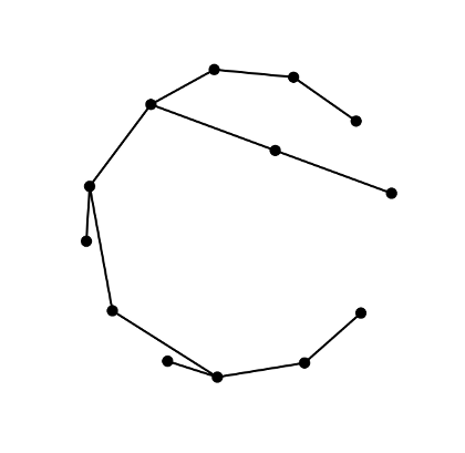
Lobsters, being trees, are planar graphs and with small lobsters plane drawings like the one above can be achieved easily. Notice that although this drawing is not an especially elegant one it does have the benefits of making both the planarity and the lobsterity of the graph clear.

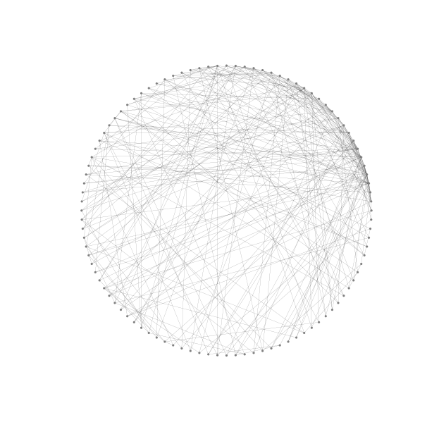
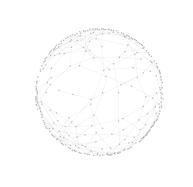
For comparison, consider the following drawing of a large lobster graph.

This drawing (the random node placement layout Gephi defaults to on loading a new graph) reveals neither the planarity nor the lobsterity of the graph.

Incidentally, the above lobster graph has 287 vertices and, being a tree, 286 edges. It was generated in Python using NetworkX. The following command creates a graph file in GEXF format (Graph Exchange Format) which can be downloaded here.

$ python -c "import networkx as nx;nx.write_gexf(nx.random_lobster(100, 0.5, 0.5, seed=0), 'lobster.gexf')"

The random_lobster(n, p, q, seed=None) function returns a lobster with approximately n vertices in the backbone, backbone edges with probability p and leaves with probability q. The seed is set to zero for the sake of reproducibility.

Force-directed drawing algorithms

The type of drawing we are looking for, one with as few edge crossings and different edge lengths as possible is the kind of drawing aimed for by force-directed algorithms. Such methods use simulations of forces between nodes to decide node placements. Electrical forces have the effect of making non-adjacent nodes move further apart and spring forces between adjacent nodes have the effect of reducing the variety of edge lengths.

Gephi makes the standard Fruchterman-Reingold force-directed algorithm available alongside a layout method unique to Gephi called Force-Atlas.

These two layout methods, although both built on force-directed foundations, produce wildly different layouts with the same lobster graph input.

Beginning with random placement of nodes, the Fruchterman-Reingold algorithm implementation in Gephi produces a layout having uniform distribution of nodes across a disk; albeit one with very many edge-crossings.

This is a well-known problem with force-directed methods. The algorithm has probably discovered a local minimum. Unfortunately this local minimum is poor in comparison with the global minimum.

The Force-Atlas algorithm, on the other hand, creates a layout which has few crossings but without the nice node distribution of the Fruchterman-Reingold layout.

One of the great benefits of Gephi is that is easy to experiment with combining these methods to produce a layout which has the benefits of both.

Combining Force-Atlas with Fruchterman-Reingold

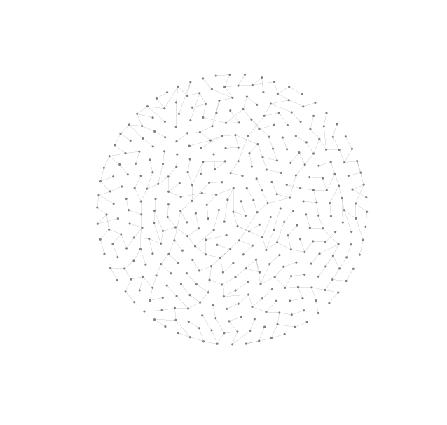
First using the Force-Atlas method to find a nearly plane drawing and then using the Fruchterman-Reingold algorithm on the resulting drawing produces a new drawing that is both nearly planar and has evenly distributed nodes with relatively few different edge lengths.

Another benefit of Gephi, not illustrated here, is that some of the layout methods allow for interaction during execution. This means that, where there are edge-crossings we can manually move vertices around a little bit to help eliminate them. So a layout like the one shown, which has few edge crossings can probably be improved to a plane drawing with a little manual interaction.

References

• Force-directed graph drawing on Wikipedia.

vis.js 2: Style Configuration

Continuing on from an earlier post, in this post we are going to look at some customisation options for vis.js.

A lot can be customised in vis.js. Some options, like those for layout, affect the entire graph. Other options, like node colours and shapes, affect nodes or groups of nodes. Yet other options, like width and style, affect edges.

As this blog is focused on graphs that arise in graph theory (as opposed to Network Analysis or other data-based disciplines) we will aim to reproduce a traditional style of graph drawing reminiscent of the simple black and white line drawings found in books and papers on graph theory. In future posts we will investigate visualisation of colouring algorithms and it will be useful to have such a default un-coloured style.

We are going to aim for the style of graph shown in this example. Black vertices, no labels, straight edges and a layout that tries to minimise edge-crossings as far as possible.

There are three steps. First we configure options related to the graph layout, then we style nodes and finally we style edges.

Graph Options

In an upcoming post we will look more closely at the different layout algorithms in vis.js and options for configuration of physics modelling that allows for dynamic interaction with the rendered graph. In this post we will settle for a layout with straight edges where nodes are placed by a repulsion algorithm.

To configure vis.js to produce such a layout involves nothing more than setting the value of two properties of the options object. This options object is then passed as a parameter to the Graph function.

The smoothCurves property has the default value of true and by changing this to false we require vis.js to use straight edges to join nodes.

The physics property supports a wide range of options but here all we want is to disable the Barnes-Hut layout algorithm and revert to a simpler repulsion layout. This is done by setting to false the value of the enabled property of the barnesHut property object.

The code below is written in CoffeeScript and we use the coffee compiler to translate it into Javascript.

options =
  smoothCurves: false
  physics:
    barnesHut:
      enabled: false

With the CoffeeScript compiler installed and the above code contained in a file called options.coffee we can produce Javascript output with:

$ coffee --compile --bare options.coffee

Then to configure all graphs in a HTML document we simply have to link to the resulting Javascript source.

For more information about graph options in vis.js see the graph options pages of the vis.js documentation.

Node Styling Options

Our goal is to have nodes rendered as black filled circles. The shape of a node is configured by setting the value of the shape property of the nodes object. The color property is a little more complicated. It allows us to specify separately the colour of the border and background of a node. We can also set different values for the border and background when the node is highlighted.

nodes:
  shape: 'circle'
  fontColor: 'black'
  color:
    border: 'black'
    background: 'black'
    highlight:
      border: 'grey'
      background: 'grey'

By choosing to have a black font colour gives a nice side-effect; labels are not visible on unhighlighted nodes. This is consistent with the graph theory setting where unlabelled graphs are prevalent.

We have opted for a subtle highlight effect by setting both border and background to grey. This colour scheme makes node labels visible when selected.

For a comprehensive list of node options see this page vis.js documentation.

Edge Styling Options

The main difference between the default styling of vis.js edges and the textbook style we are aiming to reproduce is that edges are curves instead of straight lines. To remedy this requires only that we choose the 'line' option for the style property in the edges object.

edges:
  width: 3
  style: 'line'
  color:
    color: 'black'
    highlight: 'grey'

The only other changes we have made are to increase the thickness of the edges by setting the value of the width property and choosing grey as the highlighting color of edges to match the highlighting of selected nodes.

For a comprehensive list of edge options see this page vis.js documentation.

Conclusion

The above configuration gives graph visualisations that looks something like the traditional line drawings found in graph theory literature.

For now we do not have complete control over the layout. It is generated by the repulsion algorithm and our interactions after loading the page. In future posts we will discuss how to configure both the layout algorithms and the dynamic interactions.

To learn more about the different options that can be configured in vis.js (of which we have only seen here a small sample) see the gallery on the vis.js homepage. Some examples that are particularly relevant are:

• Shapes example,
• Sizing example,
• Dashed lines example,
• Custom style example.

Source Code

References

Testing Graph Properties

Graph formats abound. As well as documented and widely-supported formats like GEXF, GML and GraphML there are as many ad-hoc or sparsely-documented formats. The latter of these usually arising as the input or output language for a standalone program implementing specific graph algorithms.

Suppose that we are trying to accomplish some task involving a graph and our task involves several steps and several different packages or programs. For an example we might be trying to colour a graph using one program, compute the graph’s automorphism group with another program and then visualise the graph using a third layout program.

In this setting we are likely to export and import our graph in multiple formats to facilitate using those different packages and we may even be forced to make ad-hoc manual or scripted changes to the file representation of the graph, for example to augment the data with vertex properties like colours or weights. Under these circumstances there is some risk that the graph file could become corrupted or invalid in some way and no longer represent the graph it claims to.

How can we be certain that a data file that purports to contain a certain graph in a specific format really does?

Testing graph properties

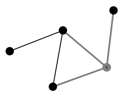
As an example, consider the Petersen graph. This graph is the smallest bridgeless cubic graph with no three-edge-colouring. We know some other properties of the Petersen graph, such as it has 10 vertices, 15 edges, radius 2, diameter 2 and girth 5. So a list of testable properties for the Petersen graph begins something like this:

• vertices 10,
• edges 15,
• radius 2,
• diameter 2,
• girth 5,
• maxdegree 3,
• …

A property testing program should be able to load a file purporting to contain a representation of the Petersen graph and test whether or not the it has these properties.

A graph failing to have all of these properties can certainly be rejected as not being the Petersen graph. A graph having enough properties in common with such a list can be said with increasing confidence, up to and beyond absolute certainty, to really be the Petersen graph.

A more extensive list of properties that the Petersen graph possesses can be found on here on Mathworld.

When it comes to storing property data for testing purposes we have at least three options. One is to store the properties with the graph in the same file. Another option is to not store the properties but to keep them in the source code of the testing program itself. A third option is to store properties externally and separately from the graph data.

In a later post we will discuss in more detail why the third of these options is preferable. For the purposes of this tutorial our properties will be kept in JSON format files. Such a file representing the above list of properties looks like this.

{
  "name": "Petersen Graph",
  "n_vertices": 10,
  "n_edges": 15,
  "radius": 2,
  "diameter": 2,
  "girth": 5,
  "maxdegree": 3,
}

In the rest of this tutorial we demonstrate how to test a file in the GML format against such a JSON list of properties.

Testing Graph Properties with CUnit

We are going to write a program in C that takes as input a property file in the above JSON format and a graph in GML format and tests whether the graph possesses the properties in the property file.

We could write a program from scratch but it benefits us to make us of a pre-existing test framework. There are many advantages to using a test framework, the most significant probably being that it greatly enhances code reuse. Another important feature of a test system built on a test framework is that all tests are run, regardless whether they succeed or fail. The testing isn’t halted by a failed test.

There are many test systems for many different languages. We restrict our attention to test systems for C of which one of the most used is CUnit.

There are several steps to creating a test program based on CUnit. In the following subsections we go through this list explaining each step in detail.

1. Get parameter data from the JSON property file.
2. Compute parameters using igraph on the graph data.
3. Express property tests as test functions.
4. Create test suites.
5. Add test suites to a registry
6. Add test functions to suites.
7. Run the tests.

Get parameter data

There are numerous choices for reading data from a JSON format file. For our purposes the library Jansson suffices.

With Jansson the properties file can be loaded with the json_load_file command

#include <jansson.h>

json_t *json = NULL;
json_error_t error;

json = json_load_file("petersen_properties.json", 0, &error)

After the property file has been loaded we use the json_object_get command to access graph properties and store them in variables to be checked later against computed parameters during the test run.

json_t *vcount_e, *ecount_e, *girth_e, *diameter_e, *maxdegree_e, *radius_e;

void get_parameter_data() {
 vcount_e = json_object_get(json, "n_vertices");
 ecount_e = json_object_get(json, "n_edges");
 radius_e = json_object_get(json, "radius");
 diameter_e = json_object_get(json, "diameter");
 girth_e = json_object_get(json, "girth");
 maxdegree_e = json_object_get(json, "maxdegree");
}

Compute parameters

The values extracted from the properties file can be thought of as expected parameter values for in the testing scenario (hence the _e suffix). Computed parameters from graph data ought to be in agreement with the expected values.

To compute parameter values from graph data there are several possibilities, including writing our own routines. In this post, however, we will make use of the extensive igraph library.

igraph provides an internal graph data structure, functions for reading the data from a file into memory and functions for computing graph parameters like those we are testing.

To load a graph from a file in GML format use the igraph_read_graph_gml.

#include <igraph.h>

igraph_t g;

i_file = fopen("petersen.gml", "r")
igraph_read_graph_gml(&g, i_file);

Once the graph itself is loaded we can then compute degree and distance parameters using the extensive functionality of igraph.

igraph_real_t radius;
igraph_integer_t diameter, girth, maxdegree;

void compute_all_parameters() {
 igraph_maxdegree(&g, &maxdegree, igraph_vss_all(), IGRAPH_ALL, IGRAPH_NO_LOOPS);
 igraph_radius(&g, &radius, IGRAPH_ALL);
 igraph_diameter(&g, &diameter, 0, 0, 0, IGRAPH_UNDIRECTED, 1);
 igraph_girth(&g, &girth, 0);
}

Express property tests

The tests themselves are expressed using CUnit’s wide range of assert macros. For our purposes we only need one of those macros, CU_ASSERT_EQUAL which tests for equality of its two arguments.

void test_basic_parameters(void)
{
 CU_ASSERT_EQUAL(igraph_vcount(&g), json_integer_value(vcount_e));
 CU_ASSERT_EQUAL(igraph_ecount(&g), json_integer_value(ecount_e));
}

void test_degree_parameters(void)
{
 CU_ASSERT_EQUAL(maxdegree, json_integer_value(maxdegree_e));
}

void test_distance_parameters(void)
{
 CU_ASSERT_EQUAL(radius, json_integer_value(radius_e));
 CU_ASSERT_EQUAL(diameter, json_integer_value(diameter_e));
 CU_ASSERT_EQUAL(girth, json_integer_value(girth_e));
}

Create test suites

The price we pay for the reusability of testing code is that there is some work to be done to set up the test suites, register them with a test runner and then run them.

The setup or init function is responsible for loading the two files. If the file-handling is successful then graph data can be read and both expected property values and actual parameters can be computed.

int init_suite(void)
{
 json_error_t error;
 if (NULL == (i_file = fopen("petersen.gml", "r")) ||
   (NULL == (json = json_load_file("petersen_properties.json", 0, &error)))) {
  return -1;
 }

 else {
  igraph_read_graph_gml(&g, i_file);
  get_parameter_data();
  compute_all_parameters();
  return 0;
 }
}

Every suite also has a teardown or clean function which is called after all of the tests in the suite have finished. This function is used to close files that need to be closed as well to initialise or destroy data structures that have been used in the tests.

int clean_suite(void)
{
 if (0 != fclose(i_file)) {
  return -1;
 }
 else {
  igraph_destroy(&g);
  i_file = NULL;
  return 0;
 }
}

Register suites

Once we have created setup and teardown functions for our test suite we must create and add the suite to the registry and give it a name. As suites correspond to graphs in this testing setting we name the suites after the graphs whose properties are under test.

CU_pSuite pSuite = CU_add_suite("Petersen Graph", init_suite, clean_suite);

Add tests to suites

With a suite created, test functions can now be added. The CU_add_test function requires the suite, a name for the test and the test itself as arguments. The test name is used in reporting the success or failure of tests.

CU_add_test(pSuite, "Basic parameters.", test_basic_parameters)
CU_add_test(pSuite, "Degree parameters.", test_degree_parameters)
CU_add_test(pSuite, "Distance parameters.", test_distance_parameters)

Run tests

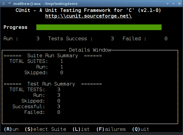
CUnit provides several test runners. There are basic, non-interactive runners as well as console and GUI-based interactive ones. On a system with Curses we can make use of an especially nice Curses-based console interface for running and monitoring the tests.

CU_basic_set_mode(CU_BRM_VERBOSE);
CU_curses_run_tests();
CU_cleanup_registry();
return CU_get_error();

When the completed test program is compiled and run the output of a successful run should look something like this:

Source Code

References