Basic Graph Drawing

In this post we introduce the drawing functionality of NetworkX.

This post is also available as a notebook for IPython which can be viewed online here.

1. Basic Drawing

All drawing in NetworkX can handled by the draw function. Layouts are generated using functions like circular_layout and spring_layout which return coordinate mappings that can be used by the draw function to render the graph.

In addition, every layout algorithm also has its own convenience function. For example, the circular layout method can be used by calling the draw_circular function and the spring layout method can be used through the draw_spring function.

In this section we will demonstrate how to use both the draw function and the different layout functions.

As with all work involving NetworkX, we have to start by importing the package. We choose to follow the popular convention to import network as nx.

import networkx as nx

NetworkX makes many named graphs available. For example, the Petersen Graph can be generated by calling the petersen_graph function.

G = nx.petersen_graph()

One way to draw the Petersen Graph with a circular layout is to pass the draw function a parameter giving the coordinates of the vertices in a circular layout. These coordinates are the output of the circular_layout function which takes the graph as a parameter.

nx.draw(G, nx.circular_layout(G))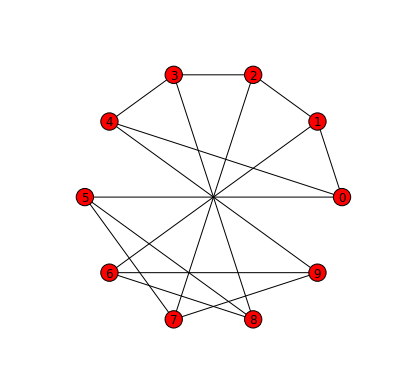

Instead of using the draw function in conjunction with the circular_layout function we can use the draw_circular convenience function.

The draw function and all of the layout convenience functions can be configured to produce graph drawings with different visual properties. Keyword parameters can be specified to customise things like node colours, edge widths and whether the graph is displayed with labels or not.

A list of all node properties that can be configured is here. A list of all edge properties that can be configured is here.

nx.draw_circular(G, with_labels=False, node_color='black')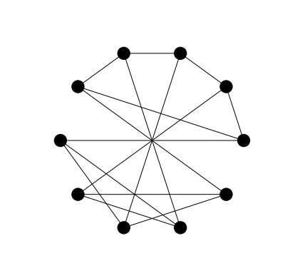

As these configuration options are going to be used on several graphs it makes sense to put all of the option configurations into a dictionary and then pass the dictionary as a parameter to the relevant layout function.

options = {
 'with_labels': False,
 'node_color': 'black',
 'node_size': 200,
 'width': 3,
}

nx.draw_circular(G, **options)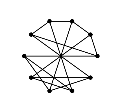

This drawing is not so easily recognised as a drawing of the Petersen Graph. A more familiar drawings shows one of the five cycles in the shape of a regular pentagon with another five cycle as a star in the interior joined to the outer cycle by five spokes. We can achieve this layout in NetworkX with the shell layout algorithm.

The draw_shell function takes an optional nlist keyword argument. The elements of the list are lists of vertices. The vertices are then arranged in concentric shells according to the elements of these lists. To find which vertices lie in the outer shell and which are in the inner shell, along with their respective orderings requires some experimentation.

nx.draw_shell(G, nlist=[range(5,10), range(5)], **options)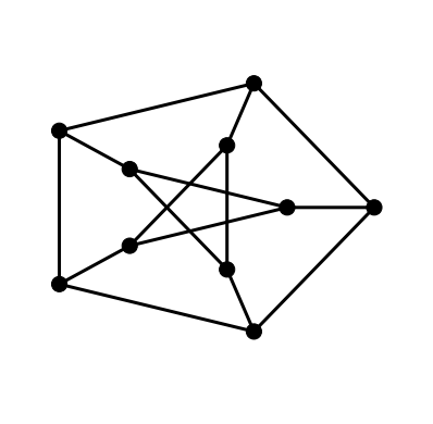

2. Simple Layouts - graphs with few vertices

NetworkX has the following layout algorithms.

• Circular
• Shell
• Spring
• Spectral
• Random
• Graphviz (through pygraphviz)

We have seen already examples of the circular and shell layouts. The next figure reproduces those two drawings from above along with examples of the spring and spectral layouts.

plt.subplot(221)
nx.draw_circular(G, **options)

plt.subplot(222)
nx.draw_shell(G, nlist=[range(5,10), range(5)], **options)

plt.subplot(223)
nx.draw_spectral(G, **options)

plt.subplot(224)
nx.draw_spring(G, **options)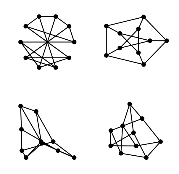

The plt.subplot command will be familiar to anyone with Matlab experience. It takes an integer argument whose first two digits are interpreted as a number of rows and columns in a rectangular grid layout and whose third argument is interpreted as the position of the current figure in the grid. Grid numbering starts in the top-left corner and proceeds right and downwards to the bottom- right corner.

3. Graphs with a few more nodes

The options we have chosen so far have been suitable for graphs with a few nodes. When we are drawing larger graphs it makes sense to choose smaller node sizes and thinner edges so that the various elements of the graph can be easily distinguished.

options_1 = {
 'with_labels': False,
 'node_color': 'black',
 'node_size': 50,
 'width': 1,
}

As with the earlier drawing of the Petersen graph the nodes for the different layers of the drawing of the dodecahedral graph below were here figured out by manual experimentation.

G = nx.dodecahedral_graph()
nx.draw_shell(G, nlist = [[2,3,4,5,6],[8,1,0,19,18,17,16,15,14,7],[9,10,11,12,13]], **options_1)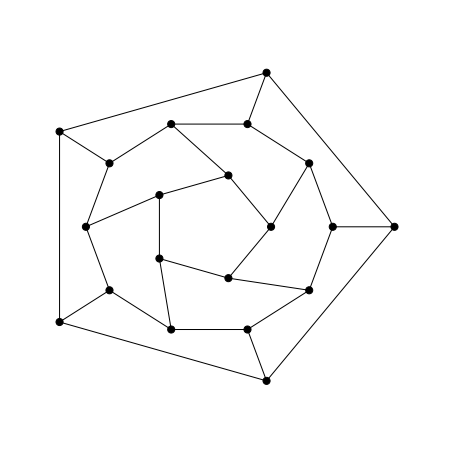

4. Graphs with many more nodes

If a graph has many nodes then there is a risk, in particular with circular or shell layouts, that node boundaries can overlap. Choosing small node sizes is a natural remedy. But when choosing very small nodes edges must also be made very thin so that we can resolve node edge intersections. Thin edges look grey and then it is natural to choose grey nodes to match.

options_2 = {
 'with_labels': False,
 'node_color': 'grey',
 'node_size': 10,
 'linewidths': 0,
 'width': 0.1,
}

G = nx.barabasi_albert_graph(100, 3)
nx.draw_circular(G, **options_2)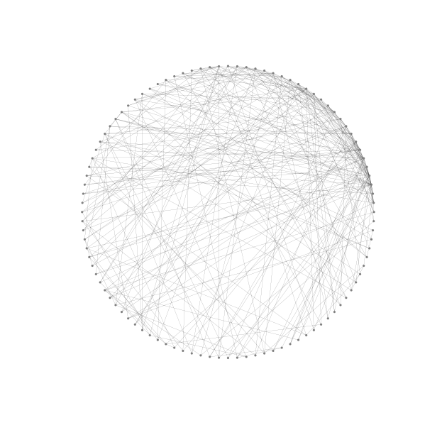

5. Graphs with many edges

Drawing graphs with many edges requires further tinkering with layout options. A new problem in this situation is that edges cannot be easily distinguished or have end vertices that are difficult to recognise. Increasing transparency by lowering the alpha value may have some benefit here.

options_3 = {
 'with_labels': False,
 'node_color': 'grey',
 'node_size': 10,
 'linewidths': 0,
 'width': 0.1,
 'alpha': 0.3
}

G = nx.complete_bipartite_graph(25,26)
nx.draw_shell(G, nlist=[range(0,25), range(25,51)], **options_3)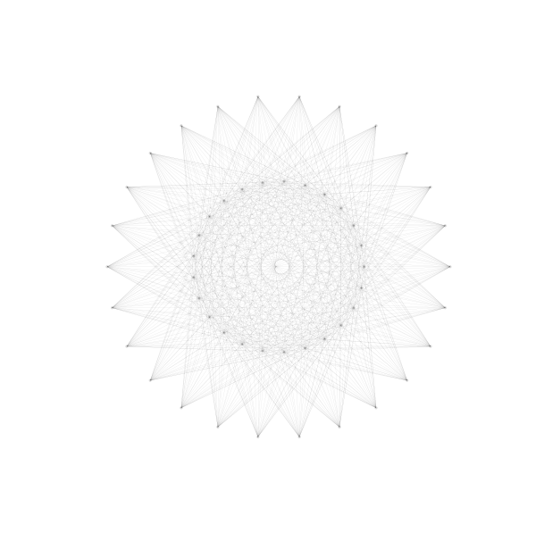

Admittedly, this drawing conveys little information about the graph. It is hard even to see which nodes in the inner shell are connected to nodes in the outer shell or if there are any connections between nodes in the inner shell. About the only information we can interpret is that nodes in the outer shell appear not to be joined to other vertices in the outer shell. Still, it serves as a basic example of the kind of issues that we face when trying to draw graphs with many edges.

4. Importing layouts from Gephi

Naturally, some of the problems encountered above are due to poorly chosen layouts. Better layouts can reduce problems of identifying nodes and edges. Even better layouts can help to highlight structural properties and symmetries of graphs.

G = nx.random_lobster(100, 0.9, 0.9)
nx.draw_spring(G, iterations=10000, **options_2)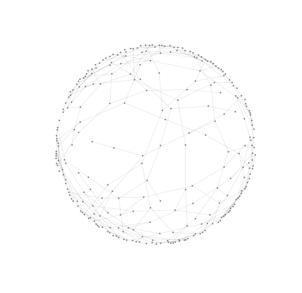

In a previous post we talked about how to use Gephi to find nice layouts of large lobster graphs. As an alternative to using NetworkX’s layout algorithms we can export our graph, use Gephi to find a suitable layout and then import the graph data back (now augmented with coordinate information) and use the raw drawing ability of NetworkX to render the graph with this layout.

G = nx.read_graphml('/home/matthew/tmp/lobster.graphml')
pos = dict([(v,(G.node[v]['x'], G.node[v]['y'])) for v in G.nodes()])

NetworkX loads the graph as a directed graph and will draw directed edges with arrows unless we set the arrows keyword argument to False.

nx.draw(G, pos, arrows=False, **options_2)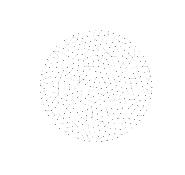

This drawing nearly has it all. The chosen layout almost conveys the planarity and lobsterity of the graph clearly. With a little manual adjustment we could eliminate all edge-crossings but because we value reproducibility above all we have left this drawing in the state generated by Gephi. Another nice property of the chosen layout is that there are few edge lengths and nodes are evenly distributed over a symmetrically shaped area, in this case a circle. Not only is the layout nice but this drawing also has suitably chosen edge widths and node sizes.