Greedy Vertex Colouring

In this post we demonstrate some of the basic ideas of vertex colouring. In particular, we demonstrate the following result.

Theorem 1

For every graph $G$, $\chi(G) \leq 1 + \Delta(G)$.

One proof of this result is found on p.182 of (Chartrand & Zhang, 2008) where it appears as Theorem 7.8. The proof is no more than a precise version of the observation that if we apply a greedy vertex colouring then we only need at most $\Delta(G) + 1$ colours because if we have that many colours then when it comes time to colour a certain vertex one is bound to be missing from the at most $\Delta(G)$ neighbours of that vertex.

Greedy Vertex Colouring

The greedy vertex colouring algorithm starts with the vertices of a graph listed in some order $v_{1},v_{2},...v_{n}$. It begins with the first vertex and assigns that vertex colour 1. To colour a vertex $v_{j + 1}$ further along in the sequence we choose the first colour which is not used on any of the already coloured vertices $\{v_{1},...v_{j}\}$.

Below is an implementation of the greedy vertex colouring algorithm for NetworkX graphs. In fact, this implementation is a little more flexible than the one described in the previous paragraph. It allows for some customisation of the algorithm’s behaviour. Specifically, it allows use to specify both the ordering of the nodes and the strategy used to select which colour to use one a particular node.

Here we have only implemented one strategy, the first_available strategy of the greedy algorithm which chooses the first colour not used on already coloured neighbours.

def first_available(G, node, palette):
    """Returns the first colour in palette which is not used in G on any
    neighbours of node, where D is the maximum degree."""
    used_on_neighbours = []
    for v in G[node]:
        used_on_neighbours.append(G.node[v].get('colour'))
    available_colour_set = set(palette) - set(used_on_neighbours)
    return sorted(available_colour_set)[0]

def vcolour(G, choose_colour = first_available, nodes = None):
    """Visits every vertex in G and assigns a colour from [0..D] given by
    the choose_colour function object, where D is the maximum degree"""
    if nodes == None:
        nodes = G.nodes()
    degseq = G.degree().values()
    if degseq!=[]:
        palette = range(max(degseq) + 1)
    else:
        palette = range(1)
    for node in nodes:
        G.node[node]['colour'] = choose_colour(G, node, palette)

Notice that this implementation colours graphs in-place. It adds a colour attribute to every vertex and the value of this attribute is the colour given to that vertex.

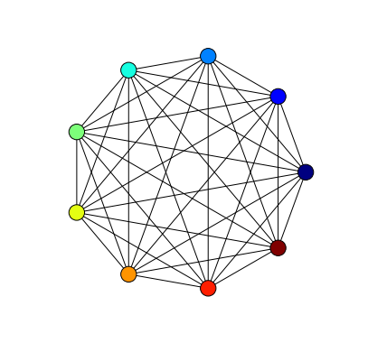
Below is an example of using the greedy colouring algorithm to colour $K_{9}$. By the earlier theorem we would expect a colouring with 9 colours, as $\Delta(K_{9}) = 8$.

import networkx as nx
setfigsize(5, 5)

options = {
 'with_labels': False,
 'node_size': 300,
 'width': 1,
}

def colours(G):
    """Returns a list of colours used on vertices in G."""
    return [x.get('colour') for x in G.node.values()]

K9 = nx.complete_graph(9)
vcolour(K9)
nx.draw_circular(K9, node_color = colours(K9), **options)

The colours function gets a list of colours used on vertices which is then passed to the draw_circular function as the argument of a keyword parameter node_colour.

We put other options into a dictionary object so that we can reuse the same options in other drawings below.

Colouring a complete graph doesn’t pose much of a challenge to any colouring algorithm. All that is needed to assign a different colour to each vertex so algorithms even simpler than the greedy algorithm will succeed in this case to find a minimal colouring.

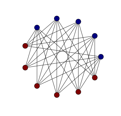
A slightly more challenging graph is a complete bipartite graph. If we consider $K_{5,6}$, for example, the above Theorem only guarantees a colouring with 7 colours. A minimal colouring, however, uses only 2 colours.

K56 = nx.complete_bipartite_graph(5,6)
vcolour(K56)
nx.draw_circular(K56, node_color = colours(K56), **options)

It isn’t really all that surprising that we found a minimal colouring here. If we have managed to colour some of the vertices properly with only two colours in such a way that all vertices of one colour lie in one of the bipartitions and all the vertices of the other colour lie in the other bipartition then it’s obvious how to extend this to a similar 2-colouring with fewer uncoloured vertices.

Colouring Some Classic Graphs

In this section we apply the greedy colouring algorithm from the previous section to some well-known graphs and compare the number of colours used with the chromatic number.

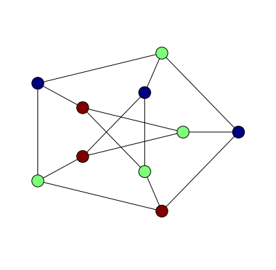
First we consider the Petersen graph. It is known to have chromatic number 3 and, indeed, with our greedy colouring algorithm we find a 3-colouring.

P = nx.petersen_graph()
vcolour(P)
nx.draw_shell(P, nlist=[range(5,10), range(5)], node_color = colours(P), **options)

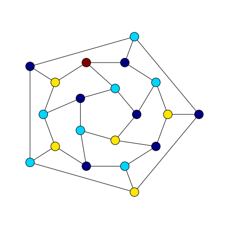
The dodecahedral graph is a slightly different story. It also has chromatic number 3 but with the greedy algorithm we find a colouring with four colours.

setfigsize(6, 6)

G = nx.dodecahedral_graph()
vcolour(G)
nlist = [[2,3,4,5,6],[8,1,0,19,18,17,16,15,14,7],[9,10,11,12,13]]
nx.draw_shell(G, nlist = nlist , node_color = colours(G), **options)

A 4-colouring of a 3-regular graph is still in accordance with Theorem 1. We might, though, do better by experimenting a little with node orderings or colour choice strategies. The first thing worth trying would be a few random orderings, hoping to hit upon one that uses only 3 colours.

random.seed(1)

G = nx.dodecahedral_graph()
nodes = G.nodes()
random.shuffle(nodes)
vcolour(G, nodes = nodes)
nlist = [[2,3,4,5,6],[8,1,0,19,18,17,16,15,14,7],[9,10,11,12,13]]
nx.draw_shell(G, nlist = nlist , node_color = colours(G), **options)

As luck would have it, we have hit upon a 3-colouring straight away, without much effort.

References

1. Chartrand, G., & Zhang, P. (2008). Chromatic Graph Theory (1st ed.). Chapman & Hall/CRC.

Processing Graph Streams

In this post we introduce gvpr a graph stream editor which belongs to the Graphviz software library. As this is our first post about Graphviz and gvpr is, perhaps, not the most obvious place to start we will begin this post with a demonstration of another program from Graphviz, gc. After that we will introduce gvpr and show how gc can be implemented in gvpr.

Our main interest in gvpr is related to last week’s post in which we were faced with the problem of applying a colouring found by Culberson’s colouring programs to a file containing graph data in DOT format. In that post we found an ad-hoc solution based on a Bash script and Sed. The approach we use here, based on gvpr, is much nicer but still might not be the best possible solution.

Counting Components with gc

GNU Coreutils, a collection of programs available on any Linux or Unix-based operating system, contains a program wc which is used to count words, lines, or characters in a document. As an example of using wc, here we calculate the number of lines, words and characters in the man page for wc.

$ man wc | wc
     70     252    2133

The Graphviz program, gc, can be thought of as a graph analogue of wc. If a graph is stored in DOT format then we can get basic metric information about the graph by invoking gc. For example, here we calculate the number of nodes in the Tutte graph.

$ curl -s https://raw.githubusercontent.com/MHenderson/graphs-collection/master/src/Classic/Tutte/tutte.gv\
  | gc -n
      46 %1 (<stdin>)

To calculate the number of edges we change the -n switch to -e:

$ curl -s https://raw.githubusercontent.com/MHenderson/graphs-collection/master/src/Classic/Tutte/tutte.gv\
  | gc -e
      69 %1 (<stdin>)

As with wc, gc can be used with multiple graphs and it will provide total counts over all input graphs.

$ curl -s https://raw.githubusercontent.com/MHenderson/graphs-collection/master/src/Classic/Tutte/tutte.gv\
   https://raw.githubusercontent.com/MHenderson/graphs-collection/master/src/Classic/Frucht/frucht.gv\
   https://raw.githubusercontent.com/MHenderson/graphs-collection/master/src/Classic/Heawood/heawood.gv\
   | gc -e
      69 %1 (<stdin>)
      18 %141 (<stdin>)
      21 %179 (<stdin>)
     108 total

gc can do some other things beside count nodes and vertices. It can also count components and clusters (which are subgraphs that are labelled as clusters). To do anything more sophisticated than merely count objects belonging to a graph we need to write another program. As we are processing text data, Sed and AWK are good choices for implementation language. Even better, though, is gvpr which has a similar approach but is designed to process data in DOT format.

gvpr - The Graph Stream Editor

gvpr is an AWK for graphs in DOT format. It is a stream editor which can be easily customised to process graph data in user-defined ways.

Implementing gc in gvpr

There are several simple examples of programs written in gvpr in the gvpr manual. One of those programs is the following gc-like program implementation. As an introduction to gvpr, in this section we will explain how this program works. The entire source code is shown below.

BEGIN { int n, e; int tot_n = 0; int tot_e = 0;}
BEG_G {
 n = nNodes($G);
 e = nEdges($G);
 printf("%d nodes %d edges %s\n", n, e, $G.name);
 tot_n += n;
 tot_e += e;
}
END { printf("%d nodes %d edges total\n", tot_n, tot_e) }

If the above code is in a file called gv and that file is located in a folder on one of the paths in the GPRPATH environment variable then we can invoke it in by calling gvpr with the filename gv as the argument of the -f switch.

$ curl -s https://raw.githubusercontent.com/MHenderson/graphs-collection/master/src/Classic/Tutte/tutte.gv\
  https://raw.githubusercontent.com/MHenderson/graphs-collection/master/src/Classic/Frucht/frucht.gv\
  https://raw.githubusercontent.com/MHenderson/graphs-collection/master/src/Classic/Heawood/heawood.gv\
  | gvpr -fgc
46 nodes 69 edges %1
12 nodes 18 edges %141
14 nodes 21 edges %179
72 nodes 108 edges total

The program works in the following way. gvpr processes the input graphs one at a time. Before doing any processing, though, it calls the action of the BEGIN clause. For our program this merely has the effect of initialising some variables we will use to count edges and vertices.

Now gvpr moves onto processing the first graph. Once it has processed the first graph it moves onto the second, and so on, until the last graph has been processed at which point it calls the action of the END clause. In our gc program this prints out the total number of edges and vertices over all of the graphs.

When gvpr processes each graph it first sets the variable $ to the current graph and then it calls the action of the BEGIN_G clause. It will then do some processing of nodes and edges (explained in the next paragraph) before calling the action of the END_G clause after each graph. In our case, when a graph is processed by gvpr we count the number of edges and vertices, print those numbers out and add them to the total edge and vertex count.

The innermost processing that gvpr does is to consider every node and edge. Any number of N and E clauses can be implemented to create some specific behaviours at nodes and edges. For example, we might provide actions to weight a node or edge with a particular value or other or we might set attributes, like the position of a vertex according to the result of a layout algorithm.

The N and E clauses both support predicate-action pairs. This means that the action will only be run if the predicate belonging to the predicate-action pair is satisfied as well as the main N or E clause (which is only true when we have encountered a node or edge).

N [ predicate ]{ action }
E [ predicate ]{ action }

In the next section we consider a different application of gvpr. We show how it can be used to take the output of a colouring from ccli and apply it to the vertices of a graph which can then be passed to one of the layout programs for drawing.

Colouring Vertices with gvpr

Our implementation of applying a colouring to a graph in DOT format in gvpr is just three lines of code.

BEG_G { setDflt($, "N", 'colorscheme', 'set13') }
N { aset($, 'style', 'filled') }
N { aset($, 'color', ARGV[$.name]) }

The basic structure is familiar from the gc-like implementation above. We have three clauses, a BEG_G clause and two N clauses. The action for each clause is a call to one of two different functions setDflt and aset.

The setDflt function sets the default value of an attribute . As we call this function in the body of the BEG_G clause the built-in variable $ is set to the current graph. In this case we are setting the default value of the colorscheme attribute for nodes to the set13 colour scheme. Graphviz provides several different colour schemes. The following quotation from the gvpr manual explains how colour schemes work.

This attribute specifies a color scheme namespace. If defined, it specifies the context for interpreting color names. In particular, if a color value has form “xxx” or “//xxx”, then the color xxx will be evaluated according to the current color scheme. If no color scheme is set, the standard X11 naming is used. For example, if colorscheme=bugn9, then color=7 is interpreted as “/bugn9/7”.

The aset function sets the value of an attribute. As we use the aset function in the body of actions that belong to N clauses we are going to be setting attributes of nodes. When gvpr is processing nodes is assigns the current node to the built-in variable $. So the syntax aset($, x, y) assigns the value y to the attribute x.

We set two attributes for every node. We set the style attribute to filled so that when the output graph is rendered by one of the drawing programs in Graphviz the nodes will be drawn as filled-in shapes, making the colour visible. The other attribute we set for each node is the color. In this case, the color is set to a value which is determined by the corresponding value of ARGV.

To use our program, call gvpr with the colour program as the argument of the -f switch. Then to provide the vertex colouring we pass a string to gvpr as the argument of the -a switch (this is then available inside of a gvpr program as the value of the ARGV variable.

gvpr -f colour -a '1 2 3 1 2 3 2 3 1 3 1 2' frucht.gv > frucht.gv.col

Now we can combine the colouring with drawing by the twopi program.

gvpr -c -f colour -a '1 2 3 1 2 3 2 3 1 3 1 2' frucht.gv |\
twopi -s\
      -Tsvg\
      -Gsize=4,4\!\
      -Groot=3\
      -Nwidth=0.3\
      -Nfixedsize=true\
      -Nlabel=\
      -Nshape=circle\
      -o frucht.svg

The resulting drawing with coloured nodes looks like this:

For more information about gvpr, a good reference is the man documentation. The source code for our program is here. The source for the above demo is here.

Drawing Coloured Queen Graphs

Continuing from last week’s post, in this post we will demonstrate how to use the osage program from Graphviz, to create rectangular drawings of coloured queen graphs. The drawings produced, like the one below, resemble coloured chess boards. Edges in these drawings are invisible but, as we will explain, it is still easy to decide whether or not the colouring of the graph is proper.

Beginning with a queen graph in DIMACS format from Michael Trick’s graph colouring instances page the goal is to produce a properly coloured queen graph in DOT format. For smaller queen graphs we can achieve colourings that use the minimal number of colours using the smallk program of Joseph Culberson. With the resulting colouring data the original DIMACS format graph data both converted into DOT format it is then a simple matter to invoke osage to produce drawings like the one above.

With the intention that others should be able to reproduce our drawings we have made available the source code in the form of several scripts and a Makefile.

The rest of this post has the following structure:

• use smallk to find a proper colouring of a small queen graph,
• convert DIMACS format queen graph into DOT format,
• generate DOT format node colouring data from smallk output,
• augment DOT graph data with DOT node colouring data,
• use osage to draw the graphs as coloured chess boards.

In an upcoming post we will return to the question of verifying, automatically, the properness of colourings.

Colouring Queen Graphs with Small Chromatic Number

In this post we consider several smaller queen graphs. Namely the $5 \times 5$, $6 \times 6$ and $7 \times 7$ queen graphs. These have, respectively, chromatic number 5,6 and 7.

One of Culberson’s graph colouring programs, smallk, is capable of properly colouring graphs with chromatic number at most 8. Consider, for example, the $5 \times 5$ queen graph. Using smallk to generate a colouring of this graph with 5 colours goes like so:

$ smallk queen5_5.col 1 5

The first argument is a randomisation seed and the second argument is the number of colours to use. If the program is successful in finding a colouring, then the output, as with all of Culberson’s colouring programs is a file that looks something like this:

CLRS 5 FROM SMALLK cpu =  0.00 pid = 23501
  2   1   5   4   3   5   4   3   2   1   3   2   1   5   4   1   5   4   3   2 
  4   3   2   1   5 

The DOT format supports vertex colouring through vertex attributes. So a conversion of this output into DOT format might begin something like this:

1 [color=red];
2 [color=blue];
3 [color=green];

Assuming a mapping of integers to colours $1\mapsto\text{blue}$, $2\mapsto\text{red}$, $5\mapsto\text{green}$ …

In the next section we demonstrate how to take this data, along with the original graph data and produce a file representing the same graph in DOT format with the vertices coloured according to a mapping of integers to colours.

Drawing Coloured Chess Boards

The drawing of our coloured queen graph will be done by osage which, like all programs belonging to the Graphviz project requires graph data to be in DOT format. In this section we show how to convert graphs from DIMACS to DOT format and then how to augment DOT format files with vertex colourings produced by smallk.

The method of this section has been implemented as Makefile which depends on several scripts introduced in the following paragraphs.

The first script dimacs2gv converts graphs from DIMACS format to DOT format. This script is little more than a sed one-liner and doubtless is neither particularly flexible nor especially robust, but suffices, at least, for our purposes and, probably, can be used in a more general setting.

When passed a graph file in DIMACS format, the output of dimacs2gv is the same graph in DOT format.

$ dimacs2gv queen5_5.col > queen5_5.gv

A second script colour takes the output of smallk and generates DOT format vertex colouring data.

$ colour queen5_5.col.res > tmp.txt

The output of colour should be added to the DOT output from dimacs2gv to produce a single file in DOT format which has all of the information, adjacency and vertex colour. The two files can be combined via sed:

$ sed -i '1r tmp.txt' queen5_5.gv

This command just says insert the contents of file tmp.txt at line 1 of the file queen5_5.gv. The -i option to sed means make the changes in-place, modifying the file directly instead of printing the result.

The DOT file now can be drawn using the osage program. There are several options to configure. The most significant of which are those that set the style of edge to invisible (-Estyle=invis) and those which make the vertices by drawn as unlabelled boxes (-Nshape=box and -Nlabel=). The other options mostly concern sizes of objects and format of output and output filename.

$ osage -s -Tsvg 
        -Gsize=5,5\! 
        -Nshape=box -Nwidth=1 -Nheight=1 -Nfixedsize=true -Nlabel=
        -Estyle=invis
         queen5_5.gv -o queen5_5.svg

The output of this command is an image in SVG format that looks something like the drawing at the beginning of this post.

Here are drawings of minimal colourings of the $6 \times 6$:

and $7 \times 7$ queen graphs:

To check these drawings for properness is easy, even though the edges are not drawn. Choose a colour and allow your eye to pick up all squares of that colour. None lie in the same row, column or diagonal. So no pair of that colour can be occupied by queens who can take each other. Doing this manually for six or seven colours only takes a few seconds. Of course, we would like to have a little program to do this automatically for us and that is a topic we will return to in a subsequent post.

Introduction to Greedy Colouring

In the post we discuss Joseph Culberson’s Graph Colouring Programs, a collection of C programs which can be downloaded from Culberson’s Graph Colouring Page.

This post has four sections. In the first, we show to use greedy in the manner it was designed to be used, interactively. In the second section we introduce a new wrapper interface, ccli, which can be used to drive greedy and the other of Culberson’s Colouring Programs in a non-interactive way which is suitable for automated experimentation and has benefits for reproducibility. In the third section we describe a general scheme for using greedy to approximate the chromatic number of graphs. In the final section we demonstrate this approach through a toy experiment into the chromatic number of queen graphs.

Interactive usage

All of Culberson’s Colouring Programs, including greedy, require input graph data to be given in DIMACS format. In this section we will demonstrate how to use greedy to find a colouring of the Chvatal Graph which can be found in DIMACS format in the graphs-collection collection of graphs.

To use greedy to colour a graph, call the program from the command-line and pass the path to the graph data in DIMACS format as an argument.

$ greedy chvatal.dimacs

After an interactive session, detailed below, the resulting colouring will be appended to a.res (where a is the original filename, including extension). This file will be created if it doesn’t already exist.

Before the colouring is produced, however, we have to participate in an interactive session with greedy to determine some options used by the program in producing the colouring. The first of these options is about whether we wish to a use a cheat colouring inside the input file as a target colouring. The purpose of this cheat is explained further in the greedy documentation. We won’t be using it here, so we respond negatively.

J. Culberson's Implementation of
        GREEDY
A program for coloring graphs.
For more information visit the webpages at:

    http://www.cs.ualberta.ca/~joe/Coloring/index.html

This program is available for research and educational purposes only.
There is no warranty of any kind.

    Enjoy!

Do you wish to use the cheat if present? (0-no, 1-yes)
0

The next option we are prompted for is a seed to be used for randomisation. This provides us with the ability to generate different random colourings and also to reproduce previously randomised colourings.

ASCII format
number of vertices = 12
p edge 12 24
Number of edges = 24 edges read = 24
GRAPH SETUP cpu =  0.00
Enter seed for search randomization:
1

Responding with 1 leads us to a choice about the type of greedy algorithm we want to use. There are six types. Again, for more information see the greedy documentation. For now we will use the simple greedy algorithm.

Process pid = 5315
GREEDY TYPE SELECTION
    1	Simple Greedy
    2	Largest First Greedy
    3	Smallest First Greedy
    4	Random Sequence Greedy
    5	Reverse Order Greedy
    6	Stir Color Greedy
Which for this program
1

The next option concerns the way in which vertices are ordered before the algorithm starts running. The default is inorder, the order vertices are given in the input graph file.

Initial Vertex Ordering:
    1 -- inorder
    2 -- random
    3 -- decreasing degree
    4 -- increasing degree
    5 -- LBFS random
    6 -- LBFS decreasing degree
    7 -- LBFS increasing degree
Using:
1

Choosing inorder for our initial vertex ordering leads us to the final option, whether or not we wish the algorithm to use the method of Kempe reductions.

Use kempe reductions y/n
n

The output is in a file called chvatal.dimacs.res and, after only one call, looks like this:

CLRS 4 FROM GREEDY cpu =  0.00 pid = 5315
  1   2   1   2   3   1   2   1   2   3   4   4

This is to be interpreted as a colouring of vertices. The first vertex gets colour 1, the second colour 2, the third colour 1 and so on. With multiple calls this file is augmented with additional lines of data in this format. This gives us a simple way of collecting information about many different runs of the same program, possibly with different options, on the same data.

Non-Interactive Use

In some situations, especially when running multiple simulations with different parameters, it can be useful to use programs non-interactively. Other benefits to this approach are that it makes it easier to chain commands together in a shell environment, for example to take the output of a colouring program and use it as part of the input to another program that draws a graph and colours nodes according to the resulting colouring. Another benefit is that it makes easier the task of documenting and communicating experimental conditions. This, in turn, can have benefits for reproducibility of results.

For this reason we have developed ccli Culberson’s (Colouring Programs) Command-Line Interface, a wrapper script around Culberson’s programs that gives them a non-interactive interface. Although still under development, ccli currently can provide a complete interface to several of the programs, including greedy.

ccli is built on docopts and expect and requires both of those programs to be installed as well as Bash 4.0 or newer.

This is the usage pattern for ccli:

ccli algorithm [options] [--] <file>...

where algorithm is one of bktdsat, dsatur, greedy, itrgreedy, maxis or tabu. The options list allows us to specify any of the same options that we would specify with the interactive interface. For example, to use the embedded cheats we add the --cheat switch to the options list. For a full explanation of all options, consult the online documentation of ccli (ccli --help).

For example, to use ccli to colour the Chvatal graph file above with the greedy algorithm of simple type with inorder vertex ordering we call ccli like so:

ccli greedy --type=simple --ordering=inorder chvatal.res

Options that are not explicitly specified on the command-line default to values which can be seen in the usage documentation (ccli --help). For example, the default for --cheat is for it to be disabled.

As before, the colouring output of this call is augmented to the chvatal.col.res file. Future versions of ccli will support output to the standard output which will allow ccli to be used in the manner of other Unix programs discussed above.

Bounds for the Chromatic Number

The greedy algorithm, both in theory and practice, is a useful tool for bounding the chromatic number of graphs. For if we have a colouring of a graph with $k$ colours then we know that the chromatic number of that graph is at most $k$.

Imagine that we have used greedy many times to produce a file a.dimacs.res which contains many different colourings of the graph a.dimacs. Then we can use a sed one-liner to extract the number of colours used by each colouring and put the results into a file.

sed -n `s/CLRS \([0-9]+\) [A-Z a-z = 0-9 .]*/\1/p` a.dimacs > output.txt

Now output.txt should contain several lines, each containing a single integer, the number of colours used in the corresponding colouring. To find the smallest of these values is just a matter of sorting the file numerically and reading the value in the first line. We put this number into a file for later inspection.

sort -n output.txt | head -n 1 > approx.txt

Now the file approx.txt contains a our best estimate for the chromatic number.

Using these little hacks we can devise a simple scheme to use ccli to estimate the chromatic number of a graph.

• Generate a large number of different colourings,
• For each colouring, compute the colouring number,
• Find the smallest colouring number over all colourings,
• Record this value as an approximation to the chromatic number.

If the colourings that we generate are all the same colouring then all of the numbers are the same. If we use Culberson’s programs in a deterministic way then we can only hope to generate a number of colourings equal to the number of combinations of algorithm and vertex orderings. Fortunately, the non-deterministic features of these programs give us the chance to generate a lot of different colourings and hopefully come up with better approximations.

The design of ccli makes it very easy to generate a lot of colourings from the shell. We simply write a loop:

!#/bin/bash
for (( i=1; i<=$1; ++i ))
do
 ccli greedy --type=$2 --ordering=$3 --seed=$RANDOM $4
done

This loop has been written in the form of a script which takes four parameters. The first is a number of iterations, the second is the algorithm type, third is the vertex ordering and the fourth is the path to the graph in DIMACS format. The $RANDOM variable is a Linux environment variable which generates a random integer and we this used to seed the random number generator in the greedy program. This means that each iteration produces a different colouring.

Bounds for the Chromatic Number of Queen Graphs

We have applied the above scheme to queen graphs. A queen graph is a graph whose vertices are the squares of a chessboard and edges join squares if and only if queens placed on those squares attack each other.

The chromatic number of queen graphs is still an open problem in general. According to the Online Encyclopedia of Integer Sequences the chromatic number of the queen graph of size 26 is unknown. Chvatal claims that in 2005 a 26-colouring of the queen graph of dimension 26 was found and thus 27 is the smallest unknown order. This follows because the chromatic number of a $n \times n$ queen graph is at least $n$ and thus a 26-colouring of the $26 \times 26$ queen graph proves that the chromatic number is 26.

In the table below we list graphs from Michael Trick’s colouring instances page. In the first column is the chromatic number, if known. Subsequent columns give approximations based on different parameters for greedy. The parameters are described in the list below the table.

The final column is the quality of the approximation, given by the ratio of the least colouring number over all colourings $\chi_{a}$ to the chromatic number $\chi$.

The source code for our experiment is available.

The columns in the above table refer to the following parameter settings:

1. --type=random --ordering=random (iterations 500)
2. --type=random --ordering=random (iterations 1000)
3. --type=random --ordering=random (iterations 5000)
4. --type=simple --ordering=random (iterations 500)
5. --type=simple --ordering=random (iterations 1000)
6. --type=simple --ordering=random (iterations 5000)
7. --type=simple --ordering=lbfsr (iterations 500)
8. --type=simple --ordering=lbfsr (iterations 1000)
9. --type=simple --ordering=lbfsr (iterations 5000) X. --type=random --ordering=lbfsd (iterations 10000)

vis.js 3: DOT Language Support and Layout Configuration

In this post we demonstrate how to take a graph stored in DOT format and draw it on a webpage using vis.js. The drawing uses vis.js’s repulsion layout algorithm and we also show how to customise this algorithm to improve the drawing in this one case.

The DOT language

The DOT graph description language is the graph format used by Graphviz, one of the oldest graph visualisation tools. More than just a library or an application, Graphviz is a large collection of tools for graph visualisation. In an upcoming series we will investigate Graphviz in detail. For a good introduction to Graphviz try Let’s Draw a Graph: An Introduction with GraphViz by Marc Khoury.

In this post our interest in the DOT language is due to the fact that vis.js can load graphs which are written in DOT.

DOT and vis.js

In the first two posts in this series we saw how to draw graphs using vis.js. In both of those posts the graph objects were created with vis.js directly with Javascript in the webpage. This is a reasonable approach for small graphs but a more common scenario is that we already have a graph contained in a file in some format and want to use the drawing algorithms of vis.js with this pre-existing graph data.

In this post we consider the above scenario under the presumption that the graph data is in DOT format. If we have graph data in a format other than DOT then we must translate it to DOT format before using vis.js. For GML this can be done with a script gml2gv in the Graphviz project (.gv being the standard file extension for files in DOT format).

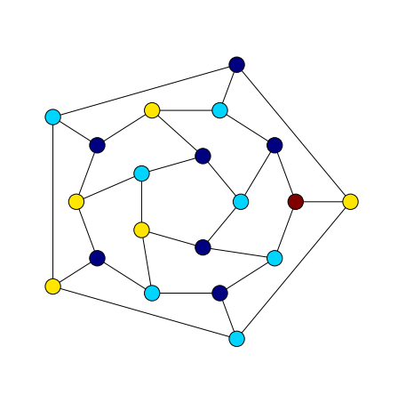
In the remainder of this post we will show how to reproduce the drawing of the dodecahedron graph (dodecahedron.gv) in the frame below.

Requesting Graph Data

To use external graph data with vis.js needs a little more work than simply calling a load or import function. The feature of vis.js that allow us to work with external data in the DOT language is the ability for the the Graph function to be initialised with a string of DOT data. So to use external data what is needed is to first create a string of DOT data from a file in DOT format.

To do this we have to make a HTTP request. This is best done asynchronously to allow graph data to be loaded while the page is being rendered. One approach is to use JQuery. Other approaches are possible but JQuery makes it very easy in this case.

$.ajax({
 url : "http://dl.dropboxusercontent.com/u/8432766/dodecahedral.gv",
 success : function(dot_str){
  var container = document.getElementById('graph');
  var graph = new vis.Graph(container, {dot: dot_str}, options);
 }
}); 

JQuery has an ajax function for making asynchronous HTTP requests. To make a GET request we simply have to provide a url string as an argument to the ajax function. In fact, because we are going to also provide other settings, it is just as easy to pack the url string as a key-value pair inside an object with other key-value pairs and pass the entire object as a parameter to the ajax function.

In this case, the only other setting required inside this parameter object is the success setting. The value of this setting is a function called when the request succeeds. The data returned by the request is passed to this function as a parameter which allows us access to the data inside the function body.

To build a Graph object from this data (called dot_str) we call the Graph function as usual but this time the second parameter, the data argument, is an object which contains a mapping from a dot key to the DOT string data which was passed into the function body when the HTTP request succeeded.

The container and options objects have been created as in previous posts. In the next section we show how to modify the options object to customise the layout of the graph so the resulting drawing is more suitable than the default.

Repulsion Layout Configuration

Layouts in vis.js are determined in a dynamic way after graph data has been loaded and thus vary from one page view to the next. Nevertheless, there are some aspects of the default drawing which are consistently undesirable and that we can fix even if we can’t completely control the exact appearance of the final graph-drawing. With default settings for the repulsion algorithm a drawing obtained by vis.js of the dodecahedron graph looks something like this:

The edges in this drawing are, arguably, too short relative to the node sizes. We can fix this by allowing the repulsion algorithm to allow nodes to be placed further apart thus making nodes appear smaller relative to the drawing size.

Several variables control the behaviour of the repulsion algorithm. These variables and their effects on the graph drawing are described in the table below, which is taken from the vis.js documentation.

A very useful feature of vis.js is an interactive interface that allows you to configure these values and then export the resulting configuration. To enable this interface just set the value of the configurePhysics option to true.

options =
  configurePhysics: true

Now when the page is viewed we are presented with the following interactive interface which can be used to experiment with different settings for the three different layout algorithms offered by vis.js.

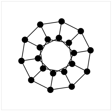
With straight edges the drawing of dodecahedron graph by the repulsion algorithm under the default variable settings has very short edges. To increase the edge length first increase the springLength setting, from 50 to 250, say. Increasing only the springLength, however, results in a poor layout because now the node distance prevents nodes from moving farther apart. The remedy is to increase node distances. 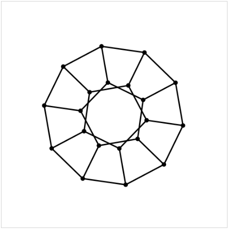Through experimentation a value of 250 for the nodeDistance gives a layout that makes the symmetry of the dodecahedron clear.

When the desired settings have been found use the Generate Options button to create option code which can be cut-and-pasted into the drawing document.

physics:
  repulsion:
   centralGravity: 0.1
   springLength: 250
   springConstant: 0.05
   nodeDistance: 250
   damping: 0.09

With those settings the drawing of the dodecahedron produced by vis.js looks something like the next image.

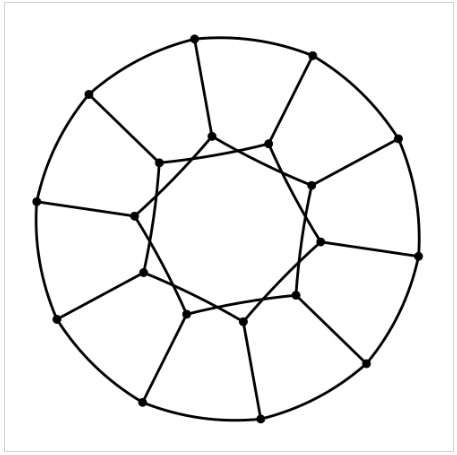
Choosing smooth curves produces a drawing with circular arcs and nearly perfect angular resolution. Such drawings are called Lombardi Drawings. See Lombardi Spirograph I: Drawing Named Graphs for further information.

Complete Source Code

The source code for the above example is shown below in a JSFiddle viewing widget. The same code is also available as a gist on Github, the output of which can be viewed on blocks.org.

Further Examples

On the vis.js homepage] this example and this playground demonstrate the use of the DOT language in vis.js.

There is also another useful example on the vis.js homepage of configuration options for the physics component of vis.js.