A Chromatic Number Program

The chromatic polynomial $\chi(G, \lambda)$ allows us to determine the chromatic number of $G$ as $\chi(G) = \min\{\lambda \in \{1,\ldots,\Delta(G) + 1\}\,|\, \chi(G, \lambda) > 0\}$

Computationally, though, the chromatic polynomial is an expensive object to construct. However, we can still use this method to calculate the chromatic numbers of small graphs.

In this blog we try to find more than one method for every calculation and for every method we try to give more than one implementation. This is because, ultimately, we hope to have reliable, reproducible results. As far as reliability goes, redundancy in our data is important and so, for this reason, here we provide another implementation of the chromatic number based on the chromatic polynomial.

In the previous post we used exclusively NetworkX for the implementation. Here we use traditional GNU utilities like Sed, cat, tr and tail, the Graphviz program gvpr, the GNU Maxima computer algebra system and an implementation of the Tutte polynomial by Haggard, Pearce and Royle.

Chromatic Numbers of Small DOT Graphs

Our program, which is little more than a wrapper script, takes as input a graph in DOT format and outputs the chromatic number. The program works by following the four steps below.

1. compute the maximum degree of the input graph,
2. convert the Graphviz data file into the input graph format used by the tutte program,
3. compute the chromatic polynomial using tutte,
4. compute the chromatic number using GNU Maxima.

The only non-trivial work here is done by the tutte and Maxima programs. Our script is simply a driver or wrapper providing a convenient interface. In fact, the dependency on GNU Maxima here could doubtless be removed because tutte is able to compute values of the polynomials it computes.

In a forthcoming post we will use the program described in this post to reproduce, and hopefully extend, the data from last week’s post on chromatic numbers of small graphs. In the rest of this post we describe each of the four steps above in detail.

Maximum Degree Computation

Some graph data formats include parameter data like number of vertices and number of edges. In this context we assume that we have a graph in DOT format without any additional parameter data. As it turns out, the tutte program infers the parameter data it needs from the graph input. So we are only left with need to calculate the maximum degree which is needed outside of tutte as the upper limit of the main loop.

A gvpr program, maxdeg computes the maximum and minimum degree of graphs in DOT format.

$ curl -s https://raw.githubusercontent.com/MHenderson/graphs-collection/master/src/Classic/Chvatal/chvatal.gv\
  | gvpr -f maxdeg
max degree = 4, node 0, min degree = 4, node 0

To use this program in our final pipeline we simply scrape out the maximum degree value from this output using Sed:

$ ...
  | sed -n 's/max degree = \([0-9]*\).*/\1/p'
4

Convert Graph Format

The input format for tutte is quite similar to the DOT format that we are using as the input format for our program. In the tutte format, edges are designated by a string of the form x--y and a graph is a comma separated list of edges.

To convert a graph in DOT format into the tutte input format can thus be accomplished by:

1. matching edges of the form x -- y; and replacing them with edges of the form x--y,,
2. removing all whitespace, including newlines,
3. removing the final, extraneous comma.

A pipeline involving Sed and tr is by no means the only way to accomplish this sequence of replacements but suffices for our purposes.

$ curl -s https://raw.githubusercontent.com/MHenderson/graphs-collection/master/src/Classic/Chvatal/chvatal.gv\
  | sed -n 's/\([0-9]*\) -- \([0-9]*\);/\1--\2,/p'\
  | tr -d ' \t\n\r\f'\
  | sed '$s/.$//'
0--1,0--4,0--6,0--9,1--2,1--5,1--7,2--3,2--6,2--8,3--4,3--7,3--9,4--5,4--8,5--10,5--11,6--10,6--11,7--8,7--11,8--10,9--10,9--11

Compute the Chromatic Polynomial

There is almost nothing to this step. We simply call the tutte program on the data from the previous step and scrape the output for the polynomial string result.

The important options for tutte in this context are --stdin which tells tutte to expect input from standard input and --chromatic which asks for the chromatic, as opposed to Tutte, polynomial.

$ curl -s https://raw.githubusercontent.com/MHenderson/graphs-collection/master/src/Classic/Chvatal/chvatal.gv
  | sed -n -e 's/\([0-9]*\) -- \([0-9]*\);/\1--\2,/p'
  | tr -d ' \t\n\r\f'| sed '$s/.$//'
  | tutte --chromatic --stdin
G[1] := {0--1,0--4,0--6,0--9,1--2,1--5,1--7,2--3,2--6,2--8,3--4,3--7,3--9,4--5,4--8,5--10,5--11,6--10,6--11,7--8,7--11,8--10,9--10,9--11}
CP[1] := -1 * x * ( 1994*(1-x) + 7427*(1-x)^2 + 12339*(1-x)^3 + 12360*(1-x)^4 + 8445*(1-x)^5 + 4191*(1-x)^6 + 1559*(1-x)^7 + 438*(1-x)^8 + 91*(1-x)^9 + 13*(1-x)^10 + 1*(1-x)^11 ) :

The chromatic polynomial is everything between G[1] := and ` : `. This delimitation makes extraction with Sed easy:

$ ...
  | sed -n 's/^CP\[1\] :=\(.*\) :/\1/p'
 -1 * x * ( 1994*(1-x) + 7427*(1-x)^2 + 12339*(1-x)^3 + 12360*(1-x)^4 + 8445*(1-x)^5 + 4191*(1-x)^6 + 1559*(1-x)^7 + 438*(1-x)^8 + 91*(1-x)^9 + 13*(1-x)^10 + 1*(1-x)^11 )

Compute the Chromatic Number

Now that we have a string representation of the chromatic polynomial we compute the chromatic number as the least positive integer for which the represented polynomial has a positive value. As $\chi(G) \leq \Delta(G) + 1$ for all graphs $G$, this can require the computation of most $\Delta(G) + 1$ values of the chromatic polynomial.

To compute a value of the chromatic polynomial from the string representation output by tutte we use the GNU Maxima computer algebra software. The at command of Maxima returns the value of its first argument polynomial string at the value of variables given in the second argument. For example, if cp is the string from the previous step then at(cp, x = 0) is the value of the polynomial represented by cp at x = 0.

m: ${max_degree}$
cp: ${cp}$
chi: for i: 1 thru m + 1 do
       if at(cp, x = i) > 0 then return (i)$
print(chi);

Maxima is an interactive program but can also be used non-interactively through the --batch or --batch-string options. The latter is sufficient for us, because our Maxima program is very short.

s="
m: ${max_degree}$
cp: ${cp}$
chi: for i: 1 thru m + 1 do
       if at(cp, x = i) > 0 then return (i)$
print(chi);"

maxima --batch-string="$s"

The default output of Maxima includes a license header and all input and output, including labels. The header can be switched off using the --very-quiet option. This option also removes the labels from input and output text. So now to scrape out the chromatic number itself we use tail to restrict our view of the output to the last line. The chromatic number is centred on this line so we remove whitespace using tr.

maxima --very-quiet --batch-string="$s"\
  | tail -n 1\
  | tr -d ' \t\r\f'

Source Code

Chromatic Polynomials

Until now we have considered two different simple methods for colouring vertices of graphs. Greedy colouring and recursive removal of independent subgraphs. Neither of which guarantee a colouring with the minimum number of colours under the most general conditions.

In the last few posts we did some simple experimentation to compare the total of chromatic numbers over all graphs on at most seven vertices against the total colours used by our greedy and recursive independent set extraction methods. This experimentation turned up some unexpected numbers and so it became necessary to investigate the data we have been using more closely so as to rule out corrupt data as a reason for the discrepancy.

We observed two things from these small experiments. Firstly, we observed that both methods used more colours than the minimum. We also observed that our NetworkX-based implementation of the greedy method appears to use many more colours than Joseph Culberson’s C version. For this reason we started to think about ways in which we could verify the data used.

As we know the distribution of chromatic numbers over small graphs, one method to verify the graph data we are using is to try to reproduce this chromatic distribution data.

In this post we therefore present an implementation of the chromatic number based on the chromatic polynomial. In upcoming posts we will return to the verification of experimental data collected in previous posts.

The Chromatic Polynomial

The chromatic polynomial $\chi_{G}(\lambda)$ is the number of $\lambda$-colourings of $G$. The chromatic polynomial is, as the name suggests, a polynomial function. To compute values of the chromatic polynomial, which can then be used to calculate the chromatic number, we will exploit the fact that it is a special case of the Tutte polynomial $T_{G}(x, y)$.

Theorem

The Tutte polynomial has been implemented by (Björklund, Husfeldt, Kaski, & Koivisto, 2008) in the tutte_bhkk module for NetworkX. Having an implementation of the Tutte polynomial, by the above Theorem, makes our job of implementing the chromatic polynomial a near triviality.

In the tutte_bhkk module there is a function tutte_poly which returns a nested list of coefficients of the Tutte polynomial. Our implementation of the chromatic polynomial will create a polynomial object rather than a coefficient list. So first we create a function that translates the tutte_bhkk coefficient list into a sympy polynomial. This is done by building a string representation of the Tutte polynomial of a graph and then using the ability of sympy.poly to construct a polynomial object from such a parameter string.

import sympy
from tutte import tutte_poly
import networkx as nx

def tutte_polynomial(G):
    T = tutte_poly(G)
    s = ' + '.join(['{0}*x**{1}*y**{2}'.format(T[i][j], i, j) for i in range(len(T)) for j in range(len(T[i]))])
    return sympy.poly(s)

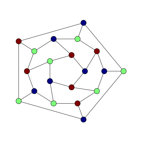
With this function now we can find, for example, the Tutte polynomial of the Petersen graph.

P = nx.petersen_graph()
tutte_polynomial(P)

With the Tutte polynomial implemented as a sympy polynomial constructing the chromatic polynomial of a graph is a no more than a simple expression. For greater convenience we embody this expression in a function, chromatic_polynomial.

from sympy.abc import x,y,l

def chromatic_polynomial(G):
    k = nx.number_connected_components(G)
    tp = tutte_polynomial(G).subs({x: 1 - l, y: 0})
    return sympy.expand((-1)**(G.number_of_nodes() - k)*l**k*tp)

Returning to the Petersen graph, the chromatic polynomial is:

cp = chromatic_polynomial(P)
cp

Now to use the chromatic polynomial to find the chromatic number of a graph it should be clear what we have to do. The Poly member function subs allows us to compute values of the chromatic polynomial. As there are no 2-colourings of the Petersen graph we expect that cp.subs(l, 2) is zero, which it is.

cp.subs(l, 2)
0

Then if we compute cp.subs(l, 3) we are not surprised to see a non-zero value because we already knew that the chromatic number of the Petersen graph is 3.

cp.subs(l, 3)
120

We see that the chromatic number of the Petersen graph is 3 because that is the least integral value of $\lambda$ for which $\chi(G, \lambda) > 0$, when $G$ is the Petersen graph.

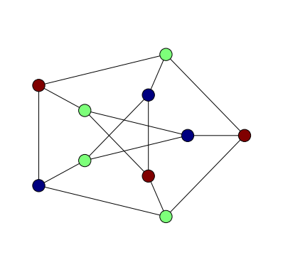
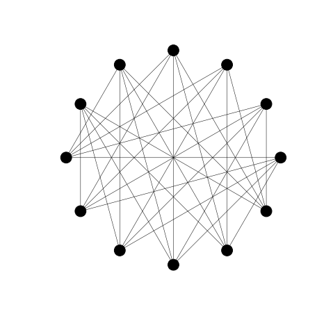
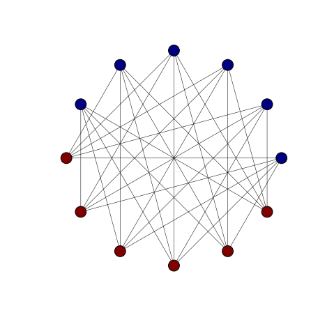
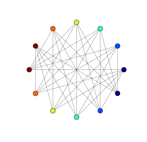
The same calculations for the Chvatal graph show that the chromatic number of the Chvatal graph is 4:

C = nx.chvatal_graph()
cp2 = chromatic_polynomial(C)

cp2.subs(l, 3)
0
cp2.subs(l, 4)
18024

Apart from some simple cases with graphs with no edge or vertices the chromatic number is found by as the least $\lambda \in \{1, \ldots, \Delta(G) + 1\}$ for which $\chi(G, \lambda) > 0$.

def chromatic_number(G):
    if G.number_of_nodes() == 0:
        return 0
    elif G.number_of_edges() == 0:
        return 1
    elif G.number_of_edges() == 1:
        return 2
    else:
        p = chromatic_polynomial(G)
        for i in range(max(G.degree().values()) + 2):
            if p.subs(l, i) > 0:
                return i

Chromatic Numbers of Small Graphs

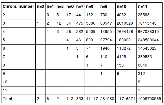
In this section we return again to the set of all graphs on at most seven vertices, albeit with more care than was given in previous posts. The first objective is to reproduce Gordon Royle’s table of chromatic numbers of small graphs as far as graphs on seven vertices. In doing this we recognise one reason for previously reported discrepant data. Royle’s table is a table of chromatic numbers for connected graphs whereas our approximations to the sum of all chromatic numbers were computed over the set of all graphs of order at most seven.

Below, we construct two lists data and c_data. The data list is populated with the chromatic number data for all graphs in the set graph_atlas_g() of all graphs on at most seven vertices. The c_data list records the same data but only for connected graphs.

from networkx.generators.atlas import graph_atlas_g
G = graph_atlas_g()

data = [8*[0] for i in range(8)]
c_data = [8*[0] for i in range(8)]

for g in G:
    n = g.number_of_nodes()
    c = chromatic_number(g)
    data[c][n] += 1
    if nx.number_connected_components(g) == 1:
        c_data[c][n] += 1

Creating a table of the distribution of chromatic numbers over all connected graphs of order at most seven we reproduce Royle’s data. The function html_table (not shown here) is based on Caleb Madrigal’s post Display List as Table in IPython Notebook.

from IPython.display import HTML

T = [['$$\chi$$','$$n = 3$$','$$n = 4$$','$$n = 5$$','$$n = 6$$','$$n = 7$$']]

rows = c_data[2:]

for i in range(len(rows)):
    R = [i + 2]
    for cell in rows[i][3:]:
      R.append(cell)
    T.append(R)

HTML(html_table(T))

The same data over all graphs of order at most seven is given in the following table.

rows = data[2:]

T = [['$$\chi$$','$$n = 3$$','$$n = 4$$','$$n = 5$$','$$n = 6$$','$$n = 7$$']]

for i in range(len(rows)):
    R = [i + 2]
    for cell in rows[i][3:]:
      R.append(cell)
    T.append(R)

HTML(html_table(T))

So this gives us some confidence in the NetworkX data as well as the above method for computing chromatic numbers.

References

1. Björklund, A., Husfeldt, T., Kaski, P., & Koivisto, M. (2008). Computing the Tutte Polynomial in Vertex-Exponential Time. In Proceedings of the 2008 49th Annual IEEE Symposium on Foundations of Computer Science (pp. 677–686). Washington, DC, USA: IEEE Computer Society. https://doi.org/10.1109/FOCS.2008.40

Vertex Colouring by Recursive Independent Set Removal

The previous two posts were about greedy colouring small graphs. In the first post an implementation of the greedy algorithm in Python with NetworkX was used to colour all graphs on at most 7 vertices. We compared different vertex orderings by counting, for different ordering strategies, the total number of colours used on this set of graphs. In the subsequent post we repeated this experiment and extended it to graphs on at most 8 vertices using Culberson’s colouring programs.

Perhaps surprisingly, Culberson’s programs did much better than our Python implementation. The most likely explanation is simply that our greedy colouring Python code is broken. Before we can conclude this, though, it is probably a good idea to investigate colouring the same set of graphs using another vertex colouring algorithm.

The goal of this post then is to introduce a slightly different approach to graph colouring, the method of recursive independent set removal.

Chromatic Numbers of Small Graphs

The minimal total number of colours used in a proper colouring of all graphs on at most seven vertices is 3348, computed from the following table which is found on Gordon Royle’s Small Graphs data page:

The total number of colours used by Culberson’s greedy program with descending degree vertex ordering was 3616. The total number of colours used by the NetworkX-based implementation was 4120.

These values differ by 504, which seems quite a large discrepancy as a proportion of the minimum of 3348 colours. What could be the cause? Or is this not a significant discrepancy? It seems to me that there are a few possibilities. The most likely explanations are problems with the data sets used in the experiments or a flaw in our implementation of the greedy algorithm. These possibilities should be eliminated first before embarking on a larger study to decide whether the discrepancy is significant or not.

Whatever are the reasons for the discrepancy it seems that some testing and verification of both graph data and colourings is in order. Seeing as we have been avoiding this issue in earlier posts it seems like an appropriate time to improve the reliability of our data.

To this end, it would be useful to have still more than implementations of vertex colouring. In this post we implement another vertex colouring algorithm based on the idea of recursively extracting a large independent set.

Colouring by Stable Set Recursion

The implementation in NetworkX of recursive maximal independent set extraction is very simple because NetworkX implements the algorithm from (Boppana & Halldórsson, 1992) in the function maximal_independent_set. Notice that this is a maximal independent set algorithm, not a maximum independent set algorithm. So at each level of recursion, we find an approximation to a maximum independent set. With small graphs this approach seems reasonably successful.

from copy import deepcopy

def __vcolour3__(G, C, level=0):
    """Vertex colouring by recursive maximal independent
       set extraction."""
    H = deepcopy(G)
    if (H.number_of_nodes() > 0):
        V1 = nx.maximal_independent_set(H)
        for v in V1: C[v]['colour'] = level
        H.remove_nodes_from(V1)
        __vcolour3__(H, C, level + 1)

def vcolour2(G):
    """Interface for vertex colouring by recursive maximal
       independent set extraction."""
    return __vcolour3__(G, G.node)

With the Petersen graph, for example, we find a minimal colouring with three colours:

import networkx as nx

P = nx.petersen_graph()
vcolour2(P)

nx.draw_shell(P, nlist = [range(5,10), range(5)], node_color = colours(P), **options)

With the dodecahedral graph we can find also a minimal 3-colouring although we have to make sure to seed the random number generator suitably.

import random
random.seed(0)

setfigsize(6, 6)

G = nx.dodecahedral_graph()
vcolour2(G)
nlist = [[2,3,4,5,6],[8,1,0,19,18,17,16,15,14,7],[9,10,11,12,13]]
nx.draw_shell(G, nlist = nlist , node_color = colours(G), **options)

We also find a minimal 4-colouring of the Grotzsch graph.

G = nx.read_graph6('/home/matthew/workspace/graphs-collection/External/HoG/graph_1132.g6')

vcolour2(G)
nx.draw_circular(G, node_color = colours(G), **options)

Colouring Small Graphs

For comparison with the colourings from the previous weeks we colour all graphs on at most seven vertices and count the total number of colours.

import networkx as nx

graphs = nx.graph_atlas_g()
colours_used = []

for G in graphs:
    vcolour2(G)
    colours_used.append(ncolours(G))
    clear_colouring(G)

sum(colours_used)
4293

This value is closer to the larger value of total colours used by our NetworkX based implementation of greedy vertex colouring. In upcoming posts we will return to the question of testing graph data so that we can rule out problems with the graph data used in these experiments.

References

1. Boppana, R., & Halldórsson, M. M. (1992). Approximating maximum independent sets by excluding subgraphs. BIT Numerical Mathematics, 32(2), 180–196. https://doi.org/10.1007/BF01994876

Improved Greedy Colouring of Small Graphs

In the previous post we conducted a small experiment to compare the total number of colours used by the greedy vertex colouring algorithm on a collection of small graphs. The aim of that experiment was to see whether, over a large number of graphs, the total number of colours used by different degree orderings was significant. The tool we used was NetworkX. In this post we revisit this experiment with Culberson’s colouring programs.

As Culberson’s implementation of the greedy colouring algorithm works with graphs in Dimacs format we need to first generate a collection of small graphs in that format. Fortunately, on the homepage of Brendan McKay there is a large collection of combinatorial data, including small graphs up to order 10. These graphs are in graph6 format but translating a graph from graph6 to Dimacs format is not too difficult thanks to some tools written by McKay for working with graphs in graph6 format.

So this is what we are going to do:

1. Download small graphs in graph6 format from BDM’s combinatorial data pages.
2. Convert all graphs from graph6 to Dimacs
3. Split file of Dimacs graphs into files, each containing one graph.
4. Colour graphs with ccli using different vertex orderings
5. Compute total colouring numbers per ordering

Convert from graph6 to Dimacs

The graph6 format is a format devised by Brendan McKay for the nauty (McKay & Piperno, 2014) graph isomorphism software. In this post we won’t attempt to describe how this format is defined. For further information see the graph6 and sparse6 graph formats page on McKay’s homepage. Gordon Royle also has some useful information about graph6 and sparse6 formats on his homepage.

The program listg (and its companion showg) which belongs to the nauty project can display graph6 graphs in various human readable formats. One format which is easy to convert into other formats is the edge format.

$ curl -s http://cs.anu.edu.au/~bdm/data/graph2.g6\
  | listg -e

Graph 1, order 2.
2 0


Graph 2, order 2.
2 1
0 1

So in graph2.g6 there are two graphs. The first graph has 2 nodes and 0 edges. The second graph has 2 nodes and 1 edge. The edge joins vertices 0 and 1.

To convert one of these files into a file of graphs in Dimacs format we use a combination of Sed and AWK. A Sed one-liner can convert a list of edges of the form x y into the x -- y form used in Dimacs. AWK will enable us to process the file of graphs in the above edge-list format and apply to Sed one-liner to each graph. The Sed one-liner in question is:

sed -r -e 's/([0-9]+) ([0-9]+)/ e \1 \2\n/g' $1

Now if we think of one of BDMs files as being made of records, each of which is a graph and consists of three lines, the third of which is the list of edges then we can use AWK to convert this into a file of DOT format graphs like so:

awk -f e2dimacs.awk output.txt > result.txt

where e2dimacs.awk is the following little snippet:

BEGIN { FS = "\n"; RS = "" }
      { print "p edge " $2 }
      { cmd="echo " $3 " | e2dimacs"; system(cmd) }

and the e2dimacs command is the above Sed one-liner.

Putting everything together into one pipeline:

$ curl -s http://cs.anu.edu.au/~bdm/data/graph2.g6\
  | listg -e\
  | awk -f e2dimacs.awk

p edge 2 0

p edge 2 1
 e 0 1

Split into individual files

Unfortunately, greedy expects that an input file contains a single graph to be coloured. This means that if we want to colour a collection of graphs in one file we have to split that file into many. One of the easiest methods is to use AWK.

Suppose we had redirected the output from the last command of the previous section into a file graph2.g6 then the following command

awk -f dimacs_split.awk graph2.dimacs

with dimacs_split.awk being the AWK program

BEGIN { FS = "\n"; RS = ""; n=0; }
      { print >> n".dimacs"; n++; }

Creates two files 0.dimacs and 1.dimacs, containing the first and second graph from the original graph6 file but now converted in Dimacs format.

Colour with greedy

At this point we have a collection of graphs each in a file of its own. We want to iterate all such files and run greedy with a specific ordering. This is easy if we know how many graphs are contained in the collection. We can just create a loop of the write length in Bash and at each step of the loop we call ccli with the correct parameters and the filename based on a loop index.

for n in {0..10};\
do\
  ccli greedy --type=simple --ordering=inorder $n.dimacs;\
done

Compute colouring numbers

The output of calling greedy on a file n.dimacs is a file n.dimacs.res in the same folder as the first file and containing the colouring data. The line preceding the colouring itself also contains the number of colours used and we can extract this number using another Sed one-liner:

sed -n 's/CLRS \([0-9]*\) [A-Z a-z = 0-9 .]*/\1/p' *.dimacs.res

The file argument here expands to a list of all files with the suffix .dimacs.res. The output is then a list of numbers, each a number of colours used in a certain colouring. We want to total all of these numbers. There are several different ways of summing numbers in a file. One convenient approach combines the paste and bc commands. The following pipeline will find all colouring numbers for a collection of files and return the total number of colours used.

sed -n 's/CLRS \([0-9]*\) [A-Z a-z = 0-9 .]*/\1/p' *.dimacs.res\
| paste -s -d"+"\
| bc

Experiment Results

We put all of the steps together into a simulation. This simulation went through all graphs of order at most 8 and computed the total number of colours used by the greedy algorithm using four different orderings. The results are given in the table below.

As before we can see that descending degree is the best way to go, at least for graphs of order at most 8.

The source code is available as a Bash script.

References

Strategies for Greedy Vertex Colourings

In the previous post we showed that a greedy vertex colouring of a graph $G$ uses at most $\Delta(G) + 1$ colours. This sounds good until we realise that graphs can have chromatic number much lower than the maximum degree.

The crown graphs, sometimes called Johnson graphs are complete bipartite graph $K_{2n, 2n}$ with a one-factor removed.

import networkx as nx

def one_factor(n):
    """The one-factor we remove from K_{2n,2n} to make a crown graph."""
    return zip(range(n),range(2*n - 1, n - 1, -1))

def crown_graph(n):
    """K_{n, n} minus one-factor."""
    G = nx.complete_bipartite_graph(n, n)
    G.remove_edges_from(one_factor(n))
    return G

G = crown_graph(6)

setfigsize(6,6)

options = {
  'with_labels': False,
  'node_size': 250,
  'width': 0.5,
}

nx.draw_circular(G, node_color = 'black', **options)

Crown graphs are bipartite and hence 2-colourable.

vcolour(G)
nx.draw_circular(G, node_color = colours(G), **options)

However, the maximum degree of a crown graph $G$ of order $2n$ is $n - 1$ and, with some vertex orderings, a greedy colouring of $G$ uses $\Delta(G) + 1 = n$ colours.

import itertools

def bad_order(n):
    """Visit nodes in the order of the missing one-factor."""
    return itertools.chain.from_iterable(one_factor(n))

clear_colouring(G)
vcolour(G, nodes = bad_order(6))
nx.draw_circular(G, node_color = colours(G), **options)

We might ask, what vertex orderings lead to colourings with fewer colours? The following theorem of Dominic A. Welsh and Martin B. Powell is pertinent.

Theorem (Welsh, Powell)

Let $G$ be a graph of order $n$ whose vertices are listed in the order $v_{1}, v_{2}, ... v_{n}$ so that $\operatorname{deg} v_{1} \geq \operatorname{deg} v_{2}\geq \dots \geq\operatorname{deg} v_{n}$. Then $\chi(G) \leq 1 + \min_{1 \leq i \leq n}\{\max{\{i - 1, \operatorname{deg} v_{i}\}\}} = \min_{1\leq i\leq n}\{\max{\{i, 1 + \operatorname{deg} v_{i}}\}\}$

In the case of regular graphs, like the crown graphs, this theorem reduces to the $\Delta(G) + 1$ upper-bound on the chromatic number. For graphs that are not regular this result suggests that we can get a tighter bound on the chromatic number by considering orderings of vertices in non-increasing degree order.

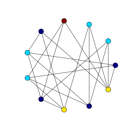
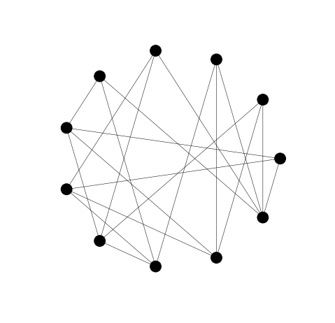
The Grotzsch graph is an irregular graph that plays an important role in the study of graph colouring. Unfortunately, it is not one of the named graphs in NetworkX. We can, however, download it from the House of Graphs as a file in graph6 format. Then we can use the read_graph6 function to read it into a NetworkX graph.

G = nx.read_graph6('/home/matthew/workspace/graphs-collection/External/HoG/graph_1132.g6')

nx.draw_circular(G, node_color = 'black', **options)

We can compute the bound from the Welsh-Powell theorem.

def welsh_powell_number(G, nodes = None):
    """Calculate bound from Welsh-Powell theorem with nodes in given order."""
    if nodes == None: nodes = G.nodes()
    if len(nodes) == 0: return 0
    else:
        return 1 + min([max(i, G.degree(nodes[i])) for i in range(len(nodes))])

welsh_powell_number(G)
4

which is a significant improvement over the $\Delta(G) + 1 = 6$ bound. In fact, the chromatic number of the Grotzsch graph is 4 and a greedy colouring with 4 colours can be found.

vcolour(G)
nx.draw_circular(G, node_color = colours(G), **options)

We might suspect then that a good vertex colouring strategy is greedy colouring with vertices in non-increasing degree order. In the next section we devise a small test of this claim.

Greedy Strategies for Colouring Small Graphs

NetworkX comes with a collection of all unlabelled, undirected graphs on seven or fewer vertices based on (Read & Wilson, 2005). The experiment below colours every graph in this collection using four different vertex orderings: in order, random order, decreasing degree order and increasing degree. In order is the order ordering of vertices in the data representation of the graph. In the case of NetworkX this just means that we colour vertices in the order they appear in G.nodes(). Random order just means that we first shuffle this list using random.shuffle. The other orderings are defined by the degree_order function below.

def degree_order(G, reverse = False):
    """Vertices of G, ordered by degree."""
    return sorted(G.nodes(), key = G.degree, reverse = reverse)

In the following code extract we iterate over the graphs in graphs_atlas_g() colouring each graph with each of the four above mentioned vertex ordering strategies. We calculate the number of colours used by each colouring and, at the end, we print out the totals of these numbers over all graphs.

import networkx as nx
import random

graphs = nx.graph_atlas_g()

colours_used = {'inorder': 0, 'random': 0, 'decdeg': 0, 'incdeg': 0}

for G in graphs:

    nodes = G.nodes()
    inorder_nodes = nodes
    random_nodes = random.shuffle(nodes)
    
    orderings = {'inorder': nodes,
                 'random': random_nodes,
                 'decdeg': degree_order(G, reverse = True),
                 'incdeg': degree_order(G)}
    
    for ordering in orderings:
        vcolour(G, nodes = orderings[ordering])
        colours_used[ordering] += ncolours(G)
        clear_colouring(G)

from IPython.display import HTML

s = """<table>
        <tr><th>Ordering</th><th>Colours used</th></tr>
        <tr><td>{0}</td><td>{1}</td></tr>
        <tr><td>{2}</td><td>{3}</td></tr>
        <tr><td>{4}</td><td>{5}</td></tr>
        <tr><td>{6}</td><td>{7}</td></tr>
       </table>"""

output = s.format('in order', colours_used['inorder'],
                  'random order', colours_used['random'],
                  'descending degree order', colours_used['decdeg'],
                  'ascending degree order', colours_used['incdeg'])

HTML(output)

We can see that the best ordering to use in this case is the ordering claimed in Welsh and Powell’s theorem. Ordering vertices by their degree from highest to lowest. The worst case is the reverse ordering and randomised and natural orderings lie somewhere in between.

References

1. Read, R. C., & Wilson, R. J. (2005). An Atlas of Graphs (Mathematics). Oxford University Press.