Chromatic Indices of Small Graphs

In this post we compute the chromatic index of all graphs on at most nine vertices with ten edges or fewer.

As in Colouring Small Graphs and Colouring Small Graphs: Update the source code for this experiment is presented as a Drakefile. As this Drakefile very similar to the Drakefiles for those earlier experiments we try to add some value by making several improvements to the quality of the source code in the hope of improving the generalisability of our method and the reproducibility of our results.

Overview

The goal is to compute the chromatic indices of all graphs whose order is at most nine. In this experiment we do part of this computation for graphs whose size is at most ten. The reason why we look at graphs with only a small number of edges is that we are using the chromatic program on the line graph $L\left(G\right)$ to compute the chromatic index ${\chi }^{\prime }\left(G\right)$ of $G$ (justified by the observation that ${\chi }^{\prime }\left(G\right)=\chi \left(L\right(G\left)\right)$). The chromatic program is slow for graphs on more than ten vertices. Therefore, as the order of $L\left(G\right)$ is equal to the size of $G$, we are restricted to graphs of small size.

As with the earlier experiments into the chromatic number, we consider connected graphs as a separate case. Also, the sets of graphs, both connected and all graphs, are sets of non-isomorphic graphs.

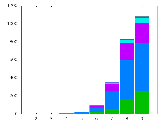
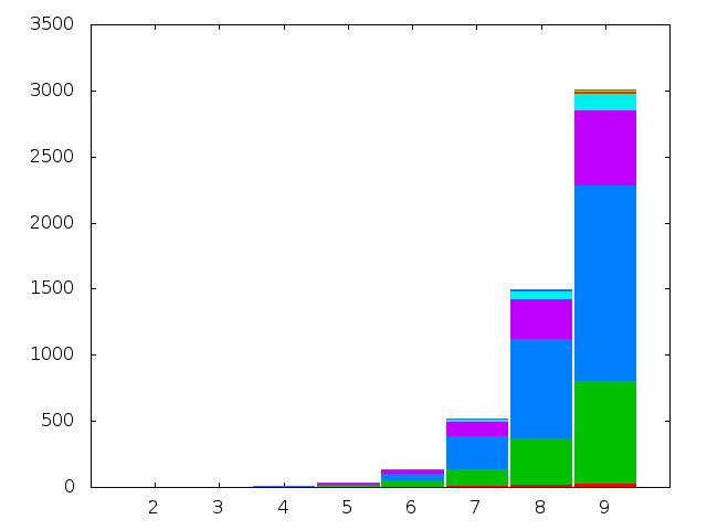
So there are two simulations whose results are presented below.

• The chromatic indices of all non-isomorphic connected simple graphs with order at most nine and size at most ten.
• The chromatic indices of all non-isomorphic simple graphs with order at most nine and size at most ten.

As things stand, we have very little in the way of verification of our results other than a little by-hand checking of total counts of graphs compared against data generated by Gordon Royle.

Experimental Details

The graph data we use is generated by geng from the gtools collection from nauty. To specify graphs of a specific size using geng we can provide the size as an optional extra argument after the order. For example, to generate all non-isomorphic connected graphs on four vertices with three edges (here piped through listg into circo for visualisation purposes):

$ geng -qc 4 3 | listg -y | circo -Tsvg -O $options

where $options was previously defined as:

$ options="-Nfixedsize=true\
           -Nlabel=\
           -Nshape=circle\
           -Nheight=0.2\
           -Nwidth=0.2\
           -Nstyle=filled\
           -Nfillcolor=black"

To generate graph data with a range of sizes an optional size argument can be given as a range in the form min:max where 0 for the upper bound is interpreted as $(\frac{n}{2})$. For example, to generate all non-isomorphic connected graphs of order four with size at least four:

$ geng -qc 4 4:0 | listg -y | circo -Tsvg -O $options

For the purposes of computing chromatic indices we transform every graph into its line graph. Line graphs can be constructed with the linegraphg program from gtools. For example, the linegraphs of the previous four graphs are:

$ geng -qc 4 4:0 | linegraphg -q | listg -y | circo -Tsvg -O $options

The -q switch for linegraphg, as with geng, suppresses auxiliary output.

As we have done in earlier experiments, we take the generated graph data in DOT format and, using csplit, split it across multiple files with one graph per file. This is done exactly as before, so we refer to the Tips and Tricks page for details.

The resulting line graph data is then processed by chromatic in the identical manner described in Colouring Small Graphs. The resulting data on the distribution of chromatic numbers (here, interpreted as chromatic indices) is then collated and tabulated, also identically as in the previously mentioned post. That distribution data is presented below in the results section along with two plots whose construction is explained now.

The table created by joining together the per-order distributions of chromatic indices is not in the perfect format for plotting with Gnuplot so a Drake rule transforms it into a new tab separated values file with an extra header row added and the final row of column totals removed.

output/data.tsv <- output/table.txt
  head -n-1 $INPUT\
  | sed -e '1i X\t2\t3\t4\t5\t6\t7\t8\t9\t' >> $OUTPUT

Another rule then transforms the above generated tsv data into a plot. The plotting is done by Gnuplot, implemented as a Drake method exploiting a little hack to pipe a Gnuplot program into Gnuplot.

plot()
  echo "\
   clear;
   reset;
   set style data histogram;
   set style histogram columnstacked;
   set style fill solid border;
   set boxwidth 0.95 relative;
   unset key;
   set term png;
   set output \"$[OUTPUT]\";
   plot for [COL=$[ORDER_MIN]:$[ORDER_MAX]] '$[INPUT]' using COL title columnheader;
  " | gnuplot

output/histogram.png <- output/data.tsv [method:plot]

The variables appearing in the Gnuplot program string are all Drake variables. The $INPUT and $OUTPUT variables are the normal automatically generated variables set when the method is called from the rule to which the method is attached. The $ORDER_MIN and $ORDER_MAX variables are set manually inside the Drakefile and are used elsewhere.

Results

• 	$n=2$	3	4	5	6	7	8	9
  $\chi =2$	0	1	2	1	2	1	2	1
  3	0	1	4	8	26	58	162	254
  4	0	0	0	10	45	193	435	538
  5	0	0	0	2	21	80	187	215
  6	0	0	0	0	0	18	39	59
  7	0	0	0	0	0	0	9	13
  8	0	0	0	0	0	0	0	4
  9	0	0	0	0	0	0	0	0
  Total:	0	2	6	21	94	350	834	1084

• 	$n=2$	3	4	5	6	7	8	9
  $\chi =2$	0	1	3	5	10	15	26	37
  3	0	1	5	14	46	123	350	772
  4	0	0	0	10	55	258	749	1476
  5	0	0	0	2	23	104	305	568
  6	0	0	0	0	0	18	57	125
  7	0	0	0	0	0	0	9	22
  8	0	0	0	0	0	0	0	4
  9	0	0	0	0	0	0	0	0
  Total:	0	2	8	31	134	518	1496	3004

Source Code

Small Moore Graphs

With geng we can generate graphs in graph6 format. For example, to generate all connected simple graphs of order four:

$ geng -qc 4
CF
CU
CV
C]
C^
C~

Here, the -q switch suppresses some auxilliary output and -c specifies connected graphs.

We can specify a class of graphs having certain properties, such as size, degree bounds, existence of cycles, connectedness or bipartiteness. For example, to generate all connected, bipartite graphs of order four with maximum degree two:

$ geng -qcb -D2 4
CU
C]

We can visualise these graphs using listg to convert the output to DOT format and the using one of the Graphviz programs to draw them. If we have many options to pass to the drawing program it makes sense to pack them all into a variable for future use.

$ options="-Nfixedsize=true\
           -Nlabel=\
           -Nshape=circle\
           -Nheight=0.2\
           -Nwidth=0.2\
           -Nstyle=filled\
           -Nfillcolor=black"

$ geng -qcb -D2 4\
  | listg -y\
  | circo -Tsvg -O $options

These two graphs answer a very easy conjecture about the existence of graphs having the following properties:

• four vertices,
• maximum degree two,
• connected,
• bipartite.

Many problems in graph theory can be expressed as the existence of graphs satisfying a list of properties like this. The existence of Moore graphs, for example, is a problem yet to be completely resolved which takes this simple form. So it might be nice to have a little program moore, that filters Moore graphs from the output of geng.

Then if we should wish, for example, to draw all Moore graphs on five vertices we can modify the above pipeline accordingly:

$ echo `geng -qc 5`
  | moore
  | listg -y
  | circo -Tsvg -O $options

In this post we show how to program such a filter in Bash and Maxima, albeit one which is fatally flawed.

Moore Graphs

A Moore graph is a graph with diameter $d$ and maximum degree $k$ which has the maximum number of vertices for a graph with the same diameter and maximum degree.

In (Cameron, 1994) it is shown that a Moore graph is any graph satisfying the following conditions (any two of which imply the third):

• $G$ is connected with maximum degree $k$ and diameter $d$;
• $G$ has minimum degree $k$ and girth $2d+1$;
• $G$ has $1+k\frac{(k-1{)}^d-1}{k-2}$ vertices.

If the output from the pipeline at the end of the previous section is correct then there are only two Moore graphs of order five, $K_5$ and $C_5$.

• $d=1$. $K_n$ and $C_3$ are the only Moore graphs.

• $d=2$. The Hoffman-Singleton theorem says that a Moore graph must have $k\in \{2,3,7,57\}$.

  • $k=2$ the unique Moore graph is $C_5$.
  • $k=3$ the unique Moore graph is the Petersen graph.
  • $k=7$ the unique Moore graph is the Hoffman-Singleton graph (shown below).
  • $k=57$ unknown whether there exists a hypothetical Moore graph which would necessarily have girth 5 and order 3250.
• $d\ge 3$. According to (Damerell, 1973) and (Bannai & Ito, 1973) the only Moore graphs is $C_{2d+1}$.

To draw the Hoffmann-Singleton graph:

$ curl http://staffhome.ecm.uwa.edu.au/~00013890/remote/cages/cagesk7g05.s6\
  | listg -y\
  | circo -Tsvg -O $options

Processing Graph Data with Maxima

The three conditions in the previous section form the basis of the Moore graph filter below. By itself we can’t use geng to identify Moore graphs because any two of these conditions involve computing either the girth or diameter.

Maxima, the computer algebra system, has a graphs library which includes functions that compute the girth and diameter of graphs. Even better, it also provides conversion to and from graph6 format.

Because the program we are going to write is supposed to work within a pipeline we will use Maxima in batch mode, rather than interactively. To avoid working with multiple source files we will use the --batch-string option to pass a program to Maxima as a string.

One drawback with Maxima is that there is a little bit of processing to be done one the output of any program because, even running in batch mode with minimal verbosity, Maxima still outputs a lot of extraneous text.

As the basic structure of the program is relatively complicated we will begin with an example. This example also serves to highlight an important consideration when it comes to the speed of the program.

In the listing below is a Bash program that calculates the degree of every graph in an input string of whitespace-delimited graphs in graph6 format.

#!/bin/bash

while read
do
 s="
 load(graphs)$
 g: graph6_decode(\"$REPLY\")$
 graph_size(g);
 "
 maxima --very-quiet --batch-string="$s"\
  | tail -n 1\
  | tr -d ' \t\r\f[]'\
  | tr ',' '\n'
done

Unfortunately, this approach is incredibly slow for at least two obvious reasons. The first is that for every graph we run a new instance of Maxima. The second is that each of these many instances of Maxima has to import the graphs library.

A different approach, which is much faster, is to read the entire list of graphs as a string, convert that string into the string representation of a Maxima list of strings and hand that to one instance of Maxima to process. The following listing does just that.

#!/bin/bash

read g6raw
g6proc=$(echo $g6raw |
         awk '{  print "\"" $1 "\"" "," }' RS=' ' ORS=' ' |
         sed '$s/. $//')
g6list="["${g6proc}"]"

s="
load(graphs)$

g6list: $g6list$
glist: map(graph6_decode, g6list)$
l:map(graph_size, glist)$
printf(true, \"~{~a,~}\", l);
"

maxima -q --very-quiet --batch-string="$s"\
 | tail -n 1\
 | tr -d ' \t\r\f'\
 | tr ',' '\n'\
 | head -n -1

This approach presents some new problems. Firstly, because we read the entire output of geng into one string we have to use echo geng. A worse problem is that we quickly run out of memory, even for very small values of the graph order. Nevertheless, for the sake of experimentation, we continue with this approach for the Moore graphs application. In the worst case it will make a reasonable base for future development.

Filtering Moore Graphs

Assuming that input is a string of whitespace-delimited graphs in graph6 format we start by building a Bash string representing a Maxima list of the same graph6 format strings.

read g6raw
g6proc=$(echo $g6raw |
         awk '{  print "\"" $1 "\"" "," }' RS=' ' ORS=' ' |
         sed '$s/. $//')
g6list="["${g6proc}"]"

The AWK program here surrounds all strings with double-quotes and adds a separating comma. The Sed hack removes the last comma and the final assignment statement puts the entire list of strings into a string surrounded by a pair of square braces, the Maxima syntax for a list.

Now we have the data in a format that can be passed to Maxima we build the entire Maxima program as a Bash string. The core of the program is a function moore1(G) which decides whether the graph G is a Moore graph or not.

moore1(G):=
 (
  K: max_degree(G)[1],
  k: min_degree(G)[1],
  d: diameter(G),
  g: girth(G),
  is_connected(G) and is(g = 2*d + 1 and k = K)
 )$

Here max_degree, min_degree, diameter, girth and is_connected are all functions from the Maxima graphs library. The is function is one of the core Maxima functions for Boolean predicate testing.

The function moore1(G) has no return statement because Maxima functions which are made up from a simple list of statements in this way return the last evaluated value by default.

For comparision, although not discussed further here, we also implemented another two functions for testing whether a graph is a Moore graph or not. These are based on the remaining two ways of choosing a pair of conditions from the list above.

moore2(g):=
 (
  k: max_degree(g)[1],
  d: diameter(g),
  expected_order: 1 + k*(((k - 1)^d - 1)/(k - 2)),
  is_connected(G) and is(graph_order(g) = expected_order)
 )$

moore3(g):=
 (
  k: min_degree(g)[1],
  d: (girth(g) - 1)/2,
  expected_order: 1 + k*(((k - 1)^d - 1)/(k - 2)),
  is(graph_order(g) = expected_order)
 )$

With the testing function implemented we turn to the graphs library and its graph6_encode and graph6_decode functions to convert the incoming data and the outgoing results.

g6list: $g6list$
glist: map(graph6_decode, g6list)$
moore_graphs: sublist(glist, moore1)$
map(graph6_encode, moore_graphs);

All of the above code is the content of a Bash string which is handed to Maxima for batch processing. This approach makes it easy, e.g g6list: $g6list to pass data from Bash to Maxima. After the Maxima program has finished we need to use tail and tr to clean up the output so that we only see the graph data and none of the auxilliary output of Maxima.

maxima --very-quiet --batch-string="$s"\
  | tail -n 1\
  | tr -d ' \t\r\f[]'\
  | tr ',' '\n'

In its present state the final script correctly identifies the Moore graphs on at most six vertices. With some improvement we hope to extend this to graphs of order at most nine.

Source Code

References

1. Cameron, P. J. (1994). Combinatorics: Topics, Techniques, Algorithms. Cambridge University Press. Retrieved from http://books.google.co.uk/books?id=xQqGQgAACAAJ
2. Damerell, R. M. (1973). On Moore graphs. Mathematical Proceedings of the Cambridge Philosophical Society, 74(02), 227–236. https://doi.org/10.1017/S0305004100048015
3. Bannai, E., & Ito, T. (1973). On finite Moore graphs. Journal of the Faculty of Science, the University of Tokyo. Sect. 1 A, Mathematics, 20(2), 191–208. Retrieved from http://ci.nii.ac.jp/naid/120000874061/en/

Colouring Small Regular Graphs

In this post we present two tables of data on chromatic numbers of regular graphs. Both tables give chromatic numbers of simple graphs on at most ten vertices. The first table shows the distribution of chromatic numbers over all regular simple graphs on at most ten vertices. The second table gives the distribution of chromatic numbers over all connected regular simple graphs on at most ten vertices. In this post we describe how this data was generated.

Overview

The method used to generate the tables is the same method using in Colouring Small Graphs except that we use geng from the gtools collection of programs from the nauty package of Brendan McKay to generate the graph data, rather than download it from McKay’s webpage. This small change has the benefit that we can now run our simulation without an internet connection. The potential disadvantage of the extra dependency on nauty is not a new disadvantage because we were already using the listg program from gtools to convert data from graph6 to DOT format.

As the method we use is almost identical to the method of Colouring Small Graphs we don’t consider all of the details again here. Instead, we will describe only the differences. These are

• using geng to generate regular graphs of order at most 10,
• splitting DOT data across multiple files using a Drake rule,
• taking a little extra care to collect chromatic numbers using grep.

Each of these small changes is discussed in detail in the following three sections. After that, we present the data itself. The source code for the entire simulation can be downloaded as a Drakefile at the bottom of the post.

Generating Regular Graphs

The small graph data available on Brendan McKay’s webpage can also be generated using the geng program.

The most basic usage pattern for geng is geng n where n is the order of graphs to be generated. The output is a listing of all graphs of order n with one graph per line in graph6 format.

$ geng 2
>A geng -d0D1 n=2 e=0-1
A?
A_
>Z 2 graphs generated in 0.00 sec

Notice that the geng 2 command was expanded automatically to geng -d0D1 n=2 e=0-1. The first and last lines here can be suppressed using the -q switch.

$ geng -q 2
A?
A_

Now this can be piped into listg -y (we can also do the piping before suppressing the auxiliary data) to convert the output graph data to DOT format.

$ geng -q 2 | listg -y
graph G1 {
}
graph G2 {
0--1;
}

The expanded call to geng which was generated automatically above is the clue to how we can use geng to generate regular graphs. Optional switches of the form -d# and -D# allow bounds on, respectively, the minimum and maximum degree to be specified. -d0D1 says that the minimum degree should be zero and the maximum degree should be 1. So, for example, to generate all 1-regular graphs on three vertices:

$ geng -q -d1D1 3
>E geng: impossible mine,maxe,mindeg,maxdeg values
>E Usage: geng [-cCmtfbd#D#] [-uygsnh] [-lvq]
              [-x#X#] n [mine[:maxe]] [res/mod] [file]
   Use geng -help to see more detailed instructions.

The error message here is no surprise. After all, there are no 1-regular graphs of order three. This reminds us that for regular graphs of odd degree we must have an even number of vertices (because the total degree $2m$ of a graph with $m$ edges is even).

$ geng -q -d1D1 4 | listg -y
graph G1 {
0--2;
1--3;
}

In this case there is only one graph because geng only generates non-isomorphic graphs.

The only other consideration we must be aware of is that if a graph is $k$-regular then, because $\Delta \left(G\right)\le n-1$, it must have at least $k+1$ vertices. So, for example, the generate all 3-regular graphs on at most ten vertices in graph6 format:

$ seq 4 2 10 | xargs -L1 geng -q -d3D3
C~
EFz_
EUxo
G?zTb_
GCrb`o
GCZJd_
GCXmd_
GCY^B_
GQhTQg
I?BeeOwM?
I?Bcu`gM?
I?bFB_wF?
I?bEHow[?
I?`bfAWF?
I?`cu`oJ?
I?`cspoX?
I?`bM_we?
I?`cm`gM?
I?`cmPoM?
I?`amQoM?
I?`c]`oM?
I?aKZ`o[?
ICOfBaKF?
ICOf@pSb?
ICOef?kF?
ICOedPKL?
ICOedO[X?
ICQRD_kQ_
ICQRD_iR?
ICQRChgI_

Piping this output (not shown) into listg -y then generates a listing of the same graphs in DOT format.

Splitting Graph Data

As before we split the resulting DOT format graph data across a folder of multiple files, one per graph. In the last post we did this outside of the Drakefile. Now, because we are generating all the graph data we use, we are forced to do the splitting with Drake.

This involves a Drake method split()

split()
  mkdir -p $OUTPUT
  csplit -sz -b '%d.gv' -f$OUTPUT/ $INPUT '/^graph.*/' '{*}'

and rules for each degree. For example, to generate the folder data/1r_gv_split from the DOT file of 1-regular graphs data/1r_gv:

data/1r_gv_split <- data/1r_gv [method:split]

The csplit invocation is exactly the same as before. The only difference in the method is that before splitting we create the output folder, if it doesn’t already exist.

Collecting Chromatic Numbers

With the graph data now built we iterate as before over all graphs, collecting their chromatic numbers. However, now because we are considering graphs of orders up to 10 there is a possibility of chromatic number 10. This means that we have to be a little bit more careful when it comes to using grep to make sure that we count occurrences of chromatic numbers correctly. Where we had been using

grep -c $j $INPUT

now we use:

grep -Fcx $j $INPUT

The -F switch here ensures that $j is considered as an entire string for matching. So, for example, if $j=10 the grep searches for occurrences of the sequence 10 not occurrences of 1 or 0. The -x switch ensures, additionally, that only exact matches are counted. For example, if 10 occurs in a longer string, 110 say, then grep won’t count this.

Results

With all of the above considerations we found the following data for regular simple graphs on at most 10 vertices, including disconnected graphs.

The data for connected regular simple graphs on at most 10 vertices is as follows:

Conclusions

At this point we haven’t given much (any?) consideration about the veracity of the above data. There is a certain degree of confidence in using a method which has been used before to generate chromatic numbers of graphs that can be verified against an existing, independent computation.

We can at least be fairly confident about the generated graph data, for a couple of reasons. Firstly, to generate the data we used a fairly trivial application of reliable graph generating software. Additionally, at least in the connected case, we can compare at least the total number of graphs of each degree against a independent computation of Markus Meringer.

In the future we will revisit the above data and consider how we might add some verification steps. There are bounds for the chromatic number of regular graphs and results like the following one of (Caccetta & Pullman, 1990) have some potential in this regard.

Theorem

If $k>1$, then for every $n\ge \lceil \frac{5k}{3}\rceil$ there is a connected, regular, $k$-chromatic graph on $n$ vertices.

One approach would be the generalise our method to graphs of greater order. The Drakefile, as it stands, is not straightforward to extend in this regard.

Source Code

References

1. Caccetta, L., & Pullman, N. J. (1990). Regular Graphs with Prescribed Chromatic Number. J. Graph Theory, 14(1), 65–71. https://doi.org/10.1002/jgt.3190140107

Colouring Small Graphs: Update

In Colouring Small Graphs we attempted to reproduce Gordon Royle’s data on the distribution of chromatic numbers of small graphs. We were partially successful, reproducing his results for graphs of order at most seven using the chromatic shell script built on the implementation of the Tutte polynomial by (Haggard, Pearce, & Royle, 2010).

Our simulation, however, ran into difficulty with graphs of order eight. We found a distribution of chromatic numbers different from Royle’s. As we had been successful with smaller orders it seemed most likely that we had some issue with corrupt data. The small graph data we started with comes from a reliable source and therefore the corruption was probably introduced by our ad-hoc methods of translating formats.

Our format conversion had two steps. We started with McKay’s graph6 format data, first converting this into Dimacs format. Then we took the Dimacs format data and converted it into Graphviz DOT format. The reason behind the two step approach was that we had previously implemented Dimacs to DOT conversion in Sed. Since then, however, we have discovered that McKay’s gtools collection of programs from the nauty (McKay & Piperno, 2014) project already implements conversion to DOT format.

The second conversion step involved splitting one file containing one graph per line into a folder of files with one graph per file. We had written an AWK program to do this but have since discovered the csplit program in the GNU Coreutils package which is specifically for this purpose.

Using these more appropriate tools has solved the problem with our reproduction of Royle’s colouring data and in this post we reproduce his table of chromatic numbers of connected graphs as far as graphs of order eight.

Overview

We start with Brendan McKay’s small graph data files in graph6 format with one graph per line and one file per order. We consider only connected graphs.

The simulation itself aims to reproduce the table of chromatic numbers of small graphs of Gordon Royle.

To reproduce the desired output we follow three steps:

1. Convert graph6 data into DOT data.
2. Process DOT data. Compute the chromatic number of every graph and store chromatic numbers in per-order results files.
3. Collate the per-order distributions into a table.

In previous posts we have tried, as far as possible, to emphasise the Unix pipeline approach to presenting a workflow. An advantage of this approach is a pipeline can be cut from the blog and pasted into a console to reproduce our simulation. A secondary benefit is that it encourages us to adhere to Unix philosophies like having small, orthogonal programs that can be combined together into pipelines to achieve more complicated tasks. We have also used Make as a more powerful language for expressing computational workflows. In this post we are going to use a Make-like tool Drake which is designed specifically for the task of expressing and automating a computational workflow. Drake is not part of GNU but it is free software.

In the rest of this post we describe each of the three steps above in more detail. At the end of this post is a Drakefile which can be used to reproduce the second two steps of our simulation. At the point of writing the data conversion step is embedded in a Makefile inside the graphs-collection project.

Convert Graph Data

This is much easier than before. The listg program in the gtools collection of programs can output graphs in DOT format by using the -y switch.

$ curl -s http://cs.anu.edu.au/~bdm/data/graph4c.g6 | listg -y
graph G1 {
0--3;
1--3;
2--3;
}
graph G2 {
0--2;
0--3;
1--3;
}
graph G3 {
0--2;
0--3;
1--3;
2--3;
}
graph G4 {
0--2;
0--3;
1--2;
1--3;
}
graph G5 {
0--2;
0--3;
1--2;
1--3;
2--3;
}
graph G6 {
0--1;
0--2;
0--3;
1--2;
1--3;
2--3;
}

Now we split this output across several files using csplit.

curl http://cs.anu.edu.au/~bdm/data/graph4c.g6
| listg -y
| csplit -sz -b '%d.gv' -f '' - '/^graph.*/' '{*}'

The result of this pipeline are six files 0.gv through 5.gv containing the six graphs above.

Options for csplit are explained in the csplit manpage and in more detail in the csplit documentation. The relevant options in this case are

• -s – Quiet output. Otherwise csplit prints out the size of each output file.
• -z – Remove empty output files.
• -b – This option has an argument describing the suffix format.
• -f – Prefix format. We have chosen an empty prefix. The default is xx.

The hyphen in the option list represents standard input. After that comes two patterns. The first is used to decide where to split. In this case we begin on any line that begins with the string graph. The second '{*}' pattern tells csplit to repeat the splitting as many times as possible.

Process Graph Data

At this point we have a collection of files in DOT format representing all connected graphs of a certain order. For each graph we compute the chromatic number, using the chromatic script, and append the result to a file of chromatic numbers of all graphs of the same order.

In this section we describe the workflow using Drake, a Make-like program designed for describing and automating computational workflows.

Drake is used by writing a Drakefile. A Drakefile bears the same relation to Drake that a Makefile bears to Make. It contains a list of rules which describe how to make an output file from an input file, collection of input files or folder.

For example, if 4c_gv is a folder containing all connected graphs of order four then a Drake rule which generates a file 4c_chromatic.txt containing the chromatic numbers of all graphs in the folder looks like this.

4c_chromatic.txt <- 4c_gv
  for graph in $INPUTS/*;
  do
   chromatic ${graph} >> $OUTPUT
  done

The assignment of 4c.gv to the variable INPUTS and 4c_chromatic.txt to the variable OUTPUT is done automatically by Drake.

The body of this rule is something that can be used in the rules for graphs of other orders. So we create a method, compute_chromatic, and assign the method to rules using the [method: compute_chromatic] rule option.

compute_chromatic()
  for graph in $INPUTS/*;
  do
   chromatic ${graph} >> $OUTPUT
  done

4c_chromatic.txt <- 4c_gv [method:compute_chromatic]

Analyse Results

The first stage of analysis is to take all the generated files of chromatic numbers and create new files containing the distribution of chromatic numbers. These files will contain two tab-separated columns. The first column being a list of possible chromatic numbers and the second being a count of graphs having that chromatic number.

For this purpose a Drake method make_distribution runs through a sequence of possible chromatic numbers. For each value grep counts the occurrences in the input file of that value and appends the result to an output file. The GNU Coreutils cut and paste are used, along with the arbitrary precision calculator language bc, to compute a total count for each chromatic number which is appended to the end of the output file.

make_distribution()
  for j in `seq 1 8`
  do
   echo -e $j'\t' `grep -c $j $INPUT` >> $OUTPUT
  done
  echo -e Total:'\t' `cut -f 2 $OUTPUT | paste -sd+ | bc` >> $OUTPUT

4c_distribution.txt <- 4c_chromatic.txt [method:make_distribution]

The second task is to take all of the distribution files (one for each order) and build a table to match the Royle table. To do this a Drake rule takes the distribution files as input and produces, as output, a file table.txt containing the table. The work is done by GNU Coreutils paste and cut which are piped together to join all distribution files into a single file and then select the relevant columns to produce the final table.

table.txt <- 2c_distribution.txt,
             3c_distribution.txt,
             4c_distribution.txt,
             5c_distribution.txt,
             6c_distribution.txt,
             7c_distribution.txt,
             8c_distribution.txt
  paste $INPUTS | cut -f 1,2,4,6,8,10,12,14 > $OUTPUT

The output of this rule is a file table.txt which contains the following table.

This table agrees with Royle’s as far as it goes. As yet we haven’t been able to extend our results to higher order because our brute-force-ish approach is too slow to process all 261080 connected graphs of order 9 in a reasonable amount of time. The good news, though, is that we have left plenty of room for improvement to the speed of our code and our approach should be ripe for parallelisation. So there is a good chance that in the future we can extend our table to match Royle’s at least as far as order 9.

Source Code

References

Colouring Small Graphs

In Chromatic Polynomials we showed how to partially reproduce the data on small graph colourings made available by Gordon Royle. In that post we used NetworkX, sympy and the tutte_bhkk module of (missing reference) to reproduce Royle’s results up to order $n=7$.

In A Chromatic Number Program we developed a tool, chromatic, for computing chromatic numbers based on tutte, an implementation of the Tutte polynomial by (Haggard, Pearce, & Royle, 2010).

In this post we attempt to reproduce Royle’s chromatic number distribution data with chromatic.

A Small Chromatic Hack

The chromatic script that we introduced last week had at least one flaw. It was not able to correctly calculate the chromatic number of a graph with no edges. This seems to be due to the fact that the input format for the tutte program used to calculate the chromatic polynomial does not support empty (i.e. edge-less) graphs.

One solution, shown below, is to calculate, using the Graphviz program gc the number of edges in the input graph. If this number is zero then we return 1 and exit the script.

n_edges=`gc -e $file_gv\
         | sed -n 's/\([0-9]*\) %.*/\1/p'\
         | tr -d ' '`

if [[ ${n_edges} -eq 0 ]] ; then
    echo 1
    exit 1
fi

Simulation Overview

Most of the work in this simulation is done by a single Bash script. In addition to looping through the graph data computing chromatic numbers we also have to first convert data into the right format and, afterwards, analyse the results.

More specifically, we have to do the following things:

1. Convert graph6 graph data from Brendan McKay’s homepage into Graphviz DOT format.
2. Iterate through all connected graphs of order at most 7 and for each graph compute the chromatic number and append it to a file of chromatic numbers of all connected graphs of the same order.
3. Analyse the distribution of chromatic numbers in the resulting results files.

In the rest of this post we describe each of these steps in more detail.

Data Conversion

We begin with the small graph data from Brendan McKay’s homepage. Among the various files he has made available are a collection which contain all graphs of order 10 or less. These are made available in graph6 format with one graph per line in files that contain all graphs of a specific order. A separate collection gives all of the connected graphs of order at most

1. The latter is the collection we are going to be using.

As things stand, chromatic, reads one graph at a time from an input file and that graph is expected to be in Graphviz DOT format. In the future it will be possible to run chromatic directly on graph6 data but for now we just do the conversion to DOT format before running the simulation.

A Makefile that converts the graph6 data into folders of files in DOT format, with one file per graph, has been added to the graphs-collection project. So to build this data we now merely clone the graphs-collection repository and call make from the src/Small folder.

Doing this creates a new folder src/Small/output which contains subfolders n_gv and nc_gv for all $2\le n\le 8$. The folder n_gv contains all graphs of order $n$ in DOT format and the folder nc_gv contains all connected graphs of order $n$ in DOT format.

The Main Loop

Once we have the data in DOT format our simulation is a very simple Bash script that takes two arguments, a lower and upper bound. The chromatic numbers of all (connected) graphs of orders between the lower and upper bounds are computed and stored in results files, one chromatic number per line, for subsequent analysis.

#!/bin/bash

BASEDIR=~/workspace/graphs-collection/src/Small/output

for order in `seq $1 $2`;
do
 echo ${order}
 graphs=`ls ${BASEDIR}/${order}c_gv/*`
 for graph in ${graphs};
 do
  chromatic ${graph} >> ${order}c_result.txt;
 done
done

The BASEDIR variable in this script points to the output folder generated in the previous step.

Analysis

A second small Bash script now is used to process the output from the previous step and collate the chromatic numbers for each order. This script also takes two parameters as input, the upper and lower bounds on order.

#!/bin/bash

RESULTS_DIR=results/14_07_31_results

for i in `seq $1 $2`
do
 echo order: $i
 for j in `seq 1 8`
 do
 echo $j: `grep -c $j ${RESULTS_DIR}/${i}c_result.txt`
 done
done

Here RESULT_DIR points to the location of the folder containing the output from the previous step

Results

The data collected by the simulation described above agrees with Royle’s table for all $n\le 6$. For $n=7$ we get the following numbers, which are obviously wrong.

We would expect that the number of connected graphs of order 7 having chromatic number 7 is (at least) 1. We also expect that there are connected graphs of order 7 having chromatic number 6. Those last two zeros, therefore, point to a flaw in our simulation.

It seems most likely that the error was introduced in converting the data from graph6 to DOT format. Our methods for converting are not designed with much rigour and it seems plausible that they aren’t reliable for larger graphs. There are at least a couple of things we can do to progress and hopefully fix this problem.

One method is to improve the reliability of our conversion tools. To do this we should match the conversions described in the Makefile in graphs-collection with some testing of basic parameters in the resulting data.

Another approach is to modify chromatic to work with files in graph6 one graph per line format.

In upcoming posts we will look at both of these approaches and return to Royle’s data with a view to reproducing his results as far as possible.

References

1. Haggard, G., Pearce, D. J., & Royle, G. (2010). Computing Tutte Polynomials. ACM Trans. Math. Softw., 37(3), 24–21. https://doi.org/10.1145/1824801.1824802