Euler Paths

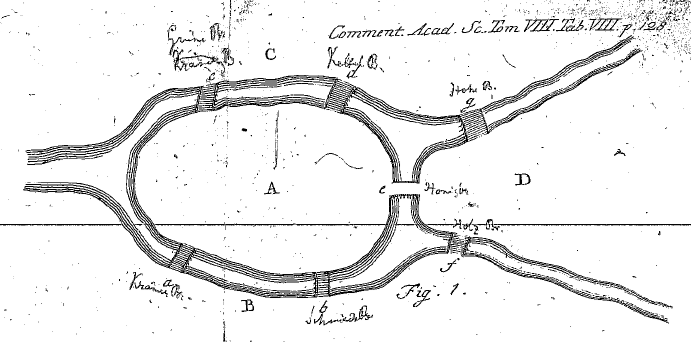
One of the oldest problems in graph theory concerns the Eastern Prussia old city of Königsberg. In that city was an island around which the river Pregel flowed in two branches. Seven bridges crossed the river to enable people to cross between mainland and island. A drawing of the river, bridges and island is shown below.

At some point the question of whether it was possible to devise a tour of the city to cross every one of the bridges once and once only was raised. In 1736, Euler showed that no such route is possible.

Euler explained his solution in (Euler, 1741) which has been translated in the first chapter of (Biggs, Lloyd, & Wilson, 1986). The original version “Solutio Problematis Ad Geometriam Situs Pertinentis” is available for download from the MAA Euler Archive.

The goal of this post is to reproduce some ideas from Euler’s paper in computer language, specifically for the Maxima computer algebra system. We describe an implementation of multigraphs in Maxima and an approach to deciding whether a path in a multigraph is an Euler path or not. In a future post we will revisit this topic and discuss searching multigraphs for Euler paths.

Multigraphs in Maxima

Maxima comes with a module for working with graphs. Unfortunately, the Maxima graphs module requires graphs to be simple, having no parallel edges and no loops. The graph which arises in the Königsberg bridges problem, however, is not simple.

One way to represent a multigraph is as a pair $G=(V,E)$ where $V$ is a set of vertices and $E$ is a set of edges. An edge ,in this context, is a pair $(e,\{u,v\left\}\right)$ where $e$ is an edge-label and $u,v$ are the end-vertices of $e$. This representation allows edges to have the same ends and only to differ in label. Loops in this setting would be pairs of the form $(e,u)$ or $(e,\{u\left\}\right)$. As none of the graphs we consider here contain loops we ignore the added complications of allowing loops.

Maxima makes it easy to create new simple data structures. The defstruct function adds a new structure to Maxima’s list of user-defined structures. A structure in Maxima has the same syntax as a function signature. The function name becomes the name of a new structure and its arguments become fields of structures of defined with new and can then be accessed with the @ syntax.

For example, we can define a graph structure like so:

(%i) defstruct(graph(V, E))$

Then a multigraph representing the bridges of Königsberg can be created like so:

(%i) konigsberg: new(graph({A,B,C,D},
                          {[a,{A,B}],
                           [b,{A,B}],
                           [c,{A,C}],
                           [d,{A,C}],
                           [e,{A,D}],
                           [f,{B,D}],
                           [g,{C,D}]}))$

The vertices of this multigraph are the regions of land, either mainland or island:

(%i) konigsberg@V;
(%o)                           {A, B, C, D}

The edges are bridges. The label of an edge being the label of the bridge in Euler’s diagram and the ends are the vertices (regions of land) joined by the bridge in question:

(%i) konigsberg@E;
(%o) [[a, {A, B}], [b, {A, B}], [c, {A, C}], [d, {A, C}],
                    [e, {A, D}], [f, {B, D}], [g, {C, D}]]

To access to the ends of a specific edge use the assoc function which gives a list or set of pairs the interface of an associative structure:

(%i) assoc(a, konigsberg@E);
(%o)                               {A, B}

Euler Paths in Maxima

A path in (Biggs, Lloyd, & Wilson, 1986) is defined as a sequence of vertices and edges $v_0,e_1,v_1,e_2,v_2,\dots ,v_{r-1},e_r,v_r$ in which each edge $e_i$ joins vertices $v_{i-1}$ and $v_i$ $(1\le i\le r)$. An Euler path is a path for which $r=|E|$, where $|E|$ is the size of the multigraph.

In Maxima paths (and non-paths) can be represented by lists of symbols. To distinguish those lists of symbols which truly represent a path in a graph we will have to check the defining properties of a path. Namely we have to be sure that

• every $v_i$ is a vertex of $G$,
• every $e_i$ is a edge of $G$,
• every $e_i$ is an edge of $G$ which joins vertices $v_{i-1}$ and $v_i$ of $G$.

As the third condition subsumes the other two and as we are only concerned with correctness here and not, yet, efficiency we can ignore the first two conditions and only check the third one.

So if $P$ is a list of symbols then $P$ is a path of multigraph $G$ if and only if

{P[i-1], P[i+1]} = assoc(P[i], G@E))

holds for all i from 2 to (length(P) - 1)/2 [lists in Maxima being indexed from 1]. This condition expresses the fact that symbols adjacent to the ith symbol are the ends of the edge represented by that symbol in some order. Notice that this condition requires that the list has the vertex-edge-vertex structure of a path.

Now we can define a function path(G, P) that decides whether $P$ is a path in $G$ or not:

path(G, P):= block(
 [result: true],
 for i: 2 step 2 thru (length(P)-1) do (
   result: result and is({P[i-1], P[i+1]} = assoc(P[i], G@E))
 ),
 return(result)
)$

With this function available, testing for Euler paths is only a matter of testing whether a path has length equal 2*length(G@E) + 1:

euler_path(G, P):= (
 is(path(G, P)) and is(length(P) = 2*length(G@E) + 1)
)$

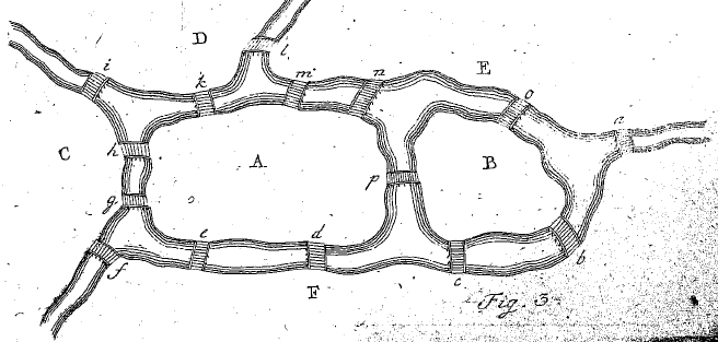
As a test of this function we check that an example of an Euler path in (Euler, 1741) really is an Euler path. As the bridges of Königsberg multigraph has on Euler path, Euler considers a fictitious map, shown below:

He claims that $EaFbBcFdAeFfCgAhCiDkAmEnApBoElD$ is an Euler path in this map. We can check by hand but now we can also represent the multigraph in Maxima and check using the above implementation of euler_path:

(%i) eulersberg: new(graph({A,B,C,D,E,F},
                          {[a,{E,F}],
                           [b,{B,F}],
                           [c,{B,F}],
                           [d,{A,F}],
                           [e,{A,F}],
                           [f,{C,F}],
                           [g,{A,C}],
                           [h,{A,C}],
                           [i,{C,D}],
                           [k,{A,D}],
                           [l,{D,E}],
                           [m,{A,E}],
                           [n,{A,E}],
                           [o,{B,E}],
                           [p,{A,B}]}))$
(%i) s: "EaFbBcFdAeFfCgAhCiDkAmEnApBoElD"
(%i) journey: map(eval_string, charlist(s))$
(%i) euler_path(eulersberg, journey);
(%o)                                true

References

1. Euler, L. (1741). Solutio problematis ad geometriam situs pertinentis. Commentarii Academiae Scientiarum Petropolitanae, 8, 128–140. Retrieved from http://www.math.dartmouth.edu/ẽuler/pages/E053.html
2. Biggs, N., Lloyd, E. K., & Wilson, R. J. (1986). Graph Theory, 1736-1936. New York, NY, USA: Clarendon Press.

More on Testing Graph Properties

In Testing Graph Properties an approach to testing graph data using CUnit is described. In this post we describe an alternative approach using Bats.

Introduction

In graphs-collection there are data files in a variety of formats that purport to represent certain graphs. Most graph formats represent graphs as list of edges or arrays of adjacencies. For even modest graphs of more than a few vertices and edges it quickly becomes difficult to verify whether certain data represents a graph in a specific format or not. For other formats, like the compressed graph6 format, human checking is practically impossible.

There are other virtues to automated tests for a collection of graph data. One significant benefit is that a collection of graph data, once verified, becomes a resource for testing graph algorithms.

Graph Property Testing

One approach to testing graph data is to have one special representation trusted to represent a specific graph and then to test other representations against this special one. In this post we take a different approach and focus on simpler, property-based testing.

Every graph has many different properties. The simplest, like order and size, might even feature as part of a data format. Others, like the chromatic number, are parameters that have to be computed from graph data by algorithms. The essence of graph property testing is to store known properties and their values as metadata and then, for every representation of a graph, check that computed values of all parameters match expected ones.

As an example, consider the following properties of the Chvatal graph, here given in YAML format.

---
name: "Chvatal Graph"
chromatic-number: 4
diameter: 2
girth: 4
max-degree: 4
order: 12
radius: 2
size: 24
...

A Bats test for the graph order is defined using the special Bats @test syntax. The body of the test itself is a sequence of shell commands. If all commands in this sequence exit with status 0 then the test passes.

@test "Chvatal graph -> graph6 -> order" {
  [ $chvatal_g6_computed_order -eq $chvatal_expected_order ]
}

The above test has a single command, a comparison between two values. If the computed order and the expected order match then this test passes. The string "Chvatal graph -> graph6 -> order" is simply a name for the test so that it can be identified in the output of Bats:

bats ./src/Classic/Chvatal/tests/*.bats
 ✓ Chvatal graph -> graph6 -> diameter
 ✓ Chvatal graph -> graph6 -> girth
 ✓ Chvatal graph -> graph6 -> order
 ✓ Chvatal graph -> graph6 -> size
 ✓ Chvatal graph -> DOT -> chi
 ✓ Chvatal graph -> DOT -> maxdeg
 ✓ Chvatal graph -> DOT -> order
 ✓ Chvatal graph -> DOT -> size

To complete the testing setup we have to implement methods to assign the values of the above variables $chvatal_g6_computed_order and $chvatal_expected_order.

The latter can be accomplished with a simple AWK program that extracts the value from the properties.yml metadata file:

cat properties.yml | awk -F": " "/order/"'{ print $2  }'

This pipeline finds the value of the order from the relevant record in the properties.yml file. As this is something that we do many time with different property files and different properties we write a function with file and property as parameters.

get_property() {
  property=$2
  s="/$property:/"'{ print $2  }'
  echo `cat $1 | awk -F": " "$s"`
}

Now, for example, the expected order can be obtained thus:

expected_order=$(get_property $properties_file order)

To compute the order of a graph from its data representation depends upon the data format used. An implementation for graphs in DOT format can be based on the gc program from Graphviz (piping the output through AWK to strip out the value of the order):

gv_order() { gc -n $1 | awk '{ print $1 }'; }

Now to compute the order from DOT data:

chvatal_gv_computed_order=$(gv_order $chvatal_gv_path)

The Petersen Graph in Diversity

In (Wester, 1994) an influential list of 123 problems that a reasonable computer algebra system (CAS) should be able to solve is presented. In this post we begin creating a similar list of problems in graph theory that a reasonable graph analysis system (GAS) ought to be able to solve.

The inspiration for this list comes from Chapter 9 of (Holton & Sheehan, 1993 ) from where the title of this post is borrowed. That chapter presents many different definitions of the Petersen graph. The aim of this post is to implement as many of them as possible. The post will be updated as more implementations are discovered.

The Petersen Graph

The Petersen graph gets its name from its appearance in the paper (Petersen, 1898) of J. Petersen as a counterexample to Tait’s claim that ‘every bridgeless cubic graph is 1-factorable’. This was not the first time the Petersen graph appeared in the literature of graph theory and far from the last. Since then it has appeared in a great many publications, often as a counterexample to a new conjecture.

Definitions of the Petersen graph arise in different ways. As direct constructions (for example by identifying antipodal points in the graph of the dodecahedron) or indirectly as one of a class of graphs satisfying certain properties (one of the bridgeless cubic graphs which are not 1-factorable).

In this post we being to collect as many different definitions as possible and give implementations of constructions or filters based on list of properties. The purpose of this is several-fold

• to initiate an effort to formulate a list of problems that a reasonable GAS ought to be able to solve,
• to motivate the development of tools for graph analysis on the command-line,
• to create test cases for a collection of graph data.

The third of these motivations is something that we will return to in future posts.

Below are two lists. The latter is a collection of properties of the Petersen graph. The first is a list of definitions. To avoid repetition, if a single property defines the Petersen graph uniquely then it appears in the first list only.

In both lists $C\left(n\right)$ denotes the set of connected cubic graphs of order $n$.

The canonical graph6 encoding of the Petersen graph is IsP@OkWHG.

The Definition List

1. The complement of the line graph of $K_5$.

       $ geng -q -d4D4 5 | linegraphg -q | complg -q | labelg -q
       IsP@OkWHG
      

1. The unique Moore graph of order 10.

       $ geng -qc 10 | moore.py | labelg -q
       IsP@OkWHG
      

1. The only graph in $C\left(10\right)$ with 120 automorphisms.

       $ geng -qc 10 -d3D3 | pickg -q -a120 | labelg -q
       IsP@OkWHG
      

1. The only graph in $C\left(10\right)$ with girth 5.

       $ paste <(geng -qc 10 -d3D3) <(geng -qc 10 -d3D3 | girth.py)\
        | awk '{ if ($2==5) print $1 }'\
        | labelg -q
       IsP@OkWHG
      

1. The only graph in $C\left(10\right)$ with diameter 2.

       $ paste <(geng -qc 10 -d3D3) <(geng -qc 10 -d3D3 | diameter.py)\
        | awk '{ if ($2==2) print $1 }'\
        | labelg -q
       IsP@OkWHG
      

1. The Kneser graph $K_{5,2}$.

       $ maxima --very-quiet --batch-string="\
          load(graphs)$
          s : powerset({`seq 1 5 | paste -s -d,`}, 2)$
          g : make_graph(s, disjointp)$
          graph6_encode(g);
         "\
         | tail -n 1\
         | tr -d ' \t\r\f'\
         | labelg -q
         IsP@OkWHG
      

1. The Odd graph $O\left(3\right)$.
2. The Moore graph with degree 3 and girth 5.
3. The graph in $C\left(10\right)$ with the most spanning trees (2000).
4. The smallest bridgeless cubic graph with no 3-edge-colouring.
5. The only bridgeless graph in $C\left(10\right)$ with chromatic number 4.
6. The only non-hamiltonian graph in $C\left(10\right)$.
7. The graph obtained from the dodecahedron graph by identifying antipodal vertices.
8. The subgraph of $G_1=\overline{T\left(7\right)}$ induced by $N\left(12\right)$.
9. The graph whose vertices are the 21 transpositions in $S_7$ whose edges join vertices that represent commuting transpositions.
10. One of only twelve connected cubic graphs with integral spectra.
11. Every orientation has diameter at least 6.
12. Every strongly connected orientation has a directed cycle of length 5.
13. Is 2-connected and all dominating cycles have length $<n$.
14. Is 1-tough $\alpha \le k+1$, $k\ge 3$ and non-hamiltonian.
15. Pancyclic and has no cycle of length 4, 5, 6 or 7 or one of two other graphs.
16. The complement of the Johnson graph $J(5,2)$.
17. As a uniform subset graph with parameters $(5,2,0)$ or $(5,3,1)$.
18. As the projective planar dual of $K_6$.
19. The unique generalised Petersen graph with $\chi =4$.

The Properties List

name – Petersen Graph

order – 10

size – 15

chromatic-number – 3

chromatic-index – 4

diameter – 2

edge-connectivity – 4

girth – 5

independence-number – 4

maximum-degree – 3

radius – 2

spectrum – $\{3,1^5,-2^4\}$

vertex-connectivity – 3

Future Directions

As of 3/10/14 there 5 of 25 definitions with full implementation. The property list contains 8 items.

Plans for the immediate future are to complete the property list and to incorporate the property list data into the testing system of the graphs-collection project.

Beyond this, the medium-term goal is to extend the list of definitions and provide implementations where possible.

In the long-term we hope to extend and generalise the list to devise a list of problems that a GAS ought to be able to solve in analogy with Wester’s list of computer algebra problems.

References

1. Wester, M. (1994). A Review of CAS Mathematical Capabilities. Computer Algebra Nederland Nieuwsbrief, 13, 41–48.
2. Holton, D. A. (D. A., & Sheehan, J. ( 1993 ). The Petersen graph . Book; Book/Illustrated , Cambridge [England] : Cambridge University Press .
3. Petersen, J. (1898). Sur le théorème de Tait. L’Intermédiaire Des Mathématiciens, 5, 225–227.

Greedy Edge Colouring of Small Graphs

In seveal earlier posts we looked at greedy vertex-colouring of small graphs. As we saw, a greedy approach to vertex-colouring is quite successful in so far as it uses at most $\Delta \left(G\right)+1$ colours to colour any graph $G$.

It is easy to modify the greedy method to colour the edges of a graph. However, we cannot guarantee that the number of colours used will be as few as $\Delta \left(G\right)+1$. The best that we can guarantee with the simplest greedy approach to edge-colouring is no more than $2\Delta \left(G\right)-1$ colours.

It’s not difficult to see why this is, for suppose that we have coloured some edges of the graph and come to colour edge $e=uv$. There might be as many as $\Delta \left(G\right)-1$ colours on edges incident with $u$ and the same amount on edges incident with $v$. In the worst case, all of these $2\Delta \left(G\right)-2$ colours might be different and so we need at least $2\Delta \left(G\right)-1$ colours in our palette to be certain, without recolouring, to have a colour available for edge $e$.

In this post we introduce a NetworkX-based implementation of greedy edge-colouring for graphs in graph6 format. Using this implementation we investigate the average case performance on all non-isomorphic, connected simple graphs of at most nine vertices. It turns out that, on average, the greedy edge-colouring method uses many fewer colours than the worst case of $2\Delta \left(G\right)-1$.

As we will discuss, the theory of edge-colouring suggests that with large sets of simple graphs we can get close, on average, to the best case of $\Delta \left(G\right)$ colours.

Greedy Edge-Colouring with NetworkX

The core of our implementation is a function that visits every edge of a graph and assigns a colour to each edge according to a parametrised colour choice strategy.

def edge_colouring(G, choice = choice_greedy):
    max_degree = max(G.degree().values())
    palette = range(0, 2*max_degree)
    for e in G.edges():
        colour_edge(G, e, choice(G, e, palette))

This function allows for some flexibility in the method used to choose the colour assigned to a certain edge. Of course, it lacks flexibility in certain other respects. For example, both the order in which edges are visited and the palette of colours are fixed.

Everything in the implementation is either Python or NetworkX, except for the colour_edge(G, e, c) and choice(G, e, p) functions. The former simply applies colour c to edge e in graph G. The latter, a function parameter that can be specified to implement different colouring strategies, decides the colour to be used.

For greedy colouring the choice strategy is plain enough. For edge $e=uv$ in graph $G$ we choose the first colour from a palette of colours which is not used on edges incident with either vertex $u$ or vertex $v$. The implementation, below, is made especially simple by Python’s Sets.

def choice_greedy(G, e, palette):
    used_colours = used_at(G, e[0]).union(used_at(G, e[1]))
    available_colours = set(palette).difference(used_colours)
    return available_colours.pop()

Here used_at(G, u) is a function that returns a Set of all colours used on edges incident with u in G. So, via the union operation on Sets, used_colours becomes the set of colours used on edges incident with end-vertices of e. The returned colours is then the colour on the top of available_colours, the set difference of palette and used_colours.

Edge-Colouring Small Graphs

The implementation described in the previous section has been put into a script that processes graphs in graph6 format and returns, not the edge-colouring, but the number of colours used. For example, the number of colours used in a greedy edge-colouring of the Petersen graph is four:

$ echo ICOf@pSb? | edge_colouring.py
4

As in earlier posts on vertex-colouring we now consider the set of all non-isomorphic, connected, simple graphs and study the average case performance of our colouring method on this set. For vertex-colouring, parallel edges have no effect on the chromatic number and thus the set of simple graphs is the right set of graphs to consider. For edge-colouring we ought to look at parallel edges and thus the set of multigraphs because parallel edges can effect the chromatic index. We will save this case for a future post.

Also in common with earlier posts, here we will use Drake as the basis for our simulation. The hope being that others can reproduce our results by downloading our Drakefile and running it.

We continue to use geng from nauty to generate the graph data we are studying. For example, to colour all non-isomorphic, connected, simple graphs on three vertices and count the colour used:

$ geng -qc 3 | edge_colouring.py
2
3

So, of the two graphs in question, one ($P_3$) has been coloured with two colours and the other ($K_3$) has been coloured with three colours.

As with vertex-colouring, the minimum number of colours in a proper edge-colouring of a graph $G$ is $\Delta \left(G\right)$. In contrast, though, by Vizing’s theorem, at most one extra colour is required.

Theorem (Vizing)

$${\chi }^{\prime }\left(G\right)\le 1+\Delta \left(G\right)$$

A graph $G$ for which ${\chi }^{\prime }\left(G\right)=\Delta \left(G\right)$ is called Class One. If ${\chi }^{\prime }\left(G\right)+1$ then $G$ is called Class Two. By Vizing’s theorem every graph is Class One or Class Two. $P_3$ is an example of a graph that is Class One and $K_3$ is an example of a Class Two graph.

Vizing’s theorem says nothing, however, about how many colours our greedy colouring program will use. We might, though, consider it moderately successful were it to use not many more than $\Delta \left(G\right)$ colours on average.

So we are going to consider the total number of colours used to colour all graphs of order $n$ as a proportion of the total maximum degree over the same set of graphs.

To compute total number of colours used we follow this tip on summing values in the console using paste and bc:

$ geng -qc 3
 | edge_colouring.py
 | paste -s -d+
 | bc
5

To compute maximum degrees we depend upon the maxdeg program for gvpr. This means that we have to pipe the output of geng through listg to convert it into DOT format:

$ geng -qc 3
 | listg -y
 | gvpr -fmaxdeg
max degree = 2, node 2, min degree = 1, node 0
max degree = 2, node 0, min degree = 2, node 0

The output from maxdeg contains much more information than we need and so we need to pipe the output through sed to strip out the maximum degrees:

$ geng -qc 3
 | listg -y
 | gvpr -fmaxdeg
 | sed -n 's/max degree = \([0-9]*\).*/\1/p'
2
2

Now, piping through paste and bc as before, we find the total over all graphs of the maximum degrees:

$ geng -qc 3
 | listg -y
 | gvpr -fmaxdeg
 | sed -n 's/max degree = \([0-9]*\).*/\1/p'
 | paste -s -d+
 | bc
4

Perhaps surprisingly, with this approach, we find a relatively small discrepancy between the total number of colours used and the total maximum degree. For example, for $n=5$ (below) the discrepancy is 18 or 25%.

$ time geng -qc 5
 | edge_colouring.py
 | paste -s -d+
 | bc
90

real	0m0.416s
user	0m0.328s
sys	0m0.068s

$ time geng -qc 5
 | listg -y
 | gvpr -fmaxdeg
 | sed -n 's/max degree = \([0-9]*\).*/\1/p'
 | paste -s -d+
 | bc
72

real	0m0.014s
user	0m0.004s
sys	0m0.004s

For $n=10$ the discrepancy is 9189586, or less than 12% of the total of maximum degrees.

$ time geng -qc 10
 | edge_colouring.py
 | paste -s -d+
 | bc
87423743

real	135m6.838s
user	131m38.614s
sys	0m12.305s

$ time geng -qc 10
 | listg -y
 | gvpr -fmaxdeg
 | sed -n 's/max degree = \([0-9]*\).*/\1/p'
 | paste -s -d+
 | bc
78234157

real	48m52.294s
user	51m43.042s
sys	0m12.737s

Results

We repeated the experiment described in the previous section for all values of $n$ from 2 to 10. The results are presented in the plot below which is based on Matplotlib basic plotting from a text file.

For all orders the total number of colours used by our greedy method is between 1 and 1.5 times the total maximum degree. There also seems to be a tendancy towards a smaller proportion for larger values of $n$. Two theoretical results are relevant here.

The first is Shannon’s theorem which concerns the chromatic index of multigraphs:

Theorem (Shannon)

$${\chi }^{\prime }\left(G\right)\le \frac{3\Delta \left(G\right)}{2}$$

Shannon’s theorem applies for our experiment because every simple graph is a multigraph with maximum multiplicity 1. An interesting experiment is to see if the results of the above experiment extend to multigraphs. Shannon’s theorem guarantees that for some colouring method it is possible but says nothing about the performance of our specific method.

A result which is relevant to the second observation, that the proportion tends to 1, concerns the distribution of simple graphs among Class One and Class Two.

Theorem (10.5 from (Chartrand & Zhang, 2008))

Almost every graph is Class One, that is ${lim}_{n\to \infty }\frac{|G_{n,1}|}{|G_n|}=1$

where $G_n$ denotes the set of graphs of order $n$ and $G_{n,1}$ is the set of Class One graphs of order $n$.

So we have good reason to hope that, on average, with larger sets of simple graphs we use fewer colours on average.

In the source code section below there is a Drakefile which should reproduce this plot from scratch (provided that the required software is installed).

Source Code

More on Moore Graphs

In Small Moore Graphs we developed moore, a filter for Moore graphs in graph6 format. The virtue of a program like moore is that it can be used in pipelines with existing programs to create new programs, as demonstrated in that earlier post.

In its present form (at time of writing) moore filters Moore graphs from a string of whitespace delimited graphs in graph6 format. So, to use it in a pipeline we have to ensure that the input is a single string, rather than raw standard input:

$ echo `geng -qc 4` | moore
C~

Beyond this small design flaw, moore has a few other, as yet unresolved, issues. For example, it fails to filter the Moore graphs of order seven from a string of all non-isomorphic connected graphs on seven vertices.

$ echo `geng -qc 7` | moore
--anerror.Todebugthistry:debugmode(true);

Rather than fix these problems immediately, in this post, we build an alternative implementation of the same program. Before, with moore we used Bash and Maxima. Here we will Python with both the NetworkX and igraph packages. The former for its graph6 handling and the latter for degree, girth and diameter calculations.

Iterating Over Graphs with Python

The resulting program, moore.py will read graphs in graph6 format from standard input and echo back those graphs which are Moore graphs.

One approach to working with standard input in Python is to use the stdin object from the sys module of the standard library. The stdin object has a readlines method that makes iterating over lines of standard input as simple as:

from sys import stdin

for line in stdin.readlines():
    # Do something

We will expect here that each line is a graph6 format string. Inside the body of the loop we then need to do the following three things:

1. parse the graph6 string into a graph object G,
2. check if G is Moore graph or not and, if it is,
3. echo the original input line on standard output.

The first of these steps can be handled by the parse_graph6 function from NetworkX. The only processing we do on each line is to strip whitespace on the right using the rstrip string method.

The result of parsing is a networkx.Graph object g. As NetworkX does not implement girth computation we construct a second igraph.Graph object G from g.edges(), the list of edges of g.

from sys import stdin

from networkx import parse_graph6

from igraph import Graph

if __name__ == "__main__":
    for line in stdin.readlines():
        stripped_line = line.rstrip()
        g = parse_graph6(stripped_line)
        G = Graph(edges = g.edges())
        moore = moore_gd
        if moore(G):
            print stripped_line

Testing for Moore graphs is done by a function moore (here pointing to one of three alternative implementations moore_gd, moore_nd and moore_gn). In the next section these three different functions are described.

Testing Moore Graphs

As seen in Small Moore Graphs there are, at least, three different ways to test whether a graph is a Moore graph or not. Those three methods are based on a theorem from (Cameron, 1994) which says that a graph is a Moore graph if it satisfies any two of the following three conditions:

1. $G$ is connected with maximum degree $k$ and diameter $d$;
2. $G$ has minimum degree $k$ and girth $2d+1$;
3. $G$ has $1+k{\sum }_{i=0}^{d-1}(k-1{)}^i$ vertices.

The third condition gives the maximum order of a $k$-regular graph with diameter $d$. As this is a value we need in more than one place it gets its own function.

def moore_order(d, k):
    """
    In a regular graph of degree k and diameter d the order is
    at most moore_order(d, k).
    """
    return 1 + k*sum([(k - 1)**i for i in range(d)])

Now moore_gn, which is based on the combination of conditions 2 (involving girth) and 3 (involving order) above can be implemented for igraph.Graph objects as follows:

def moore_gn(G):
  """
  Decide if G is a Moore graph or not, based on order and girth.
  """
  return G.vcount() == moore_order((G.girth() - 1)/2, min(G.degree()))

Remembering that every graph which satisfies conditions 2 and 3 above is also regular and connected might persuade us to consider some optimisations here. For example, as the minimum degree of vertices must be calculated we might as well also compute the maximum degree and avoid moore_order and girth calculations for any graph for which those values differ.

Similarly, we might also dismiss any graph which isn’t connected. Optimisations like these require some experimentation to determine their worth. Also, when programs like geng have already efficient ways to generated connected and regular graphs there will be circumstances when we only want the essential computation to be done. So at present we will concentrate on building a reliable implementation and leave such considerations for the future.

With disregard for optimisation in mind, the other testing functions based on the remaining combinations of conditions 1, 2 and 3. are also very simple one-liners. The girth and diameter variant looks like:

def moore_gd(G):
  """
  Decide if G is a Moore graph or not, based on girth and diameter.
  """
  return G.girth() == 2*G.diameter() + 1

While the version based on order and diameter is:

def moore_nd(G):
  """
  Decide if G is a Moore graph or not, based on order and diameter.
  """
  return G.vcount() == moore_order(G.diameter(), max(G.degree()))

Results

Now we can construct all Moore graphs on at most 10 vertices in a single pipeline involving geng and moore.py. Here the resulting graphs are visualised with circo from Graphviz after conversion to DOT format using listg:

$ options="-Gsize=5,5!
           -Nfixedsize=true
           -Nlabel=
           -Nshape=circle
           -Nheight=0.2
           -Nwidth=0.2
           -Nstyle=filled
           -Nfillcolor=black"

$ seq 1 10\
  | xargs -L1 geng -qc\
  | moore.py\
  | listg -y\
  | circo -Tsvg -O $options

The video below demonstrates the use of moore.py and compares it with the program moore described in Small Moore Graphs

Source Code

References

1. Cameron, P. J. (1994). Combinatorics: Topics, Techniques, Algorithms. Cambridge University Press. Retrieved from http://books.google.co.uk/books?id=xQqGQgAACAAJ